12 Workflow: Visium CRC

12.1 Preamble

12.1.1 Introduction

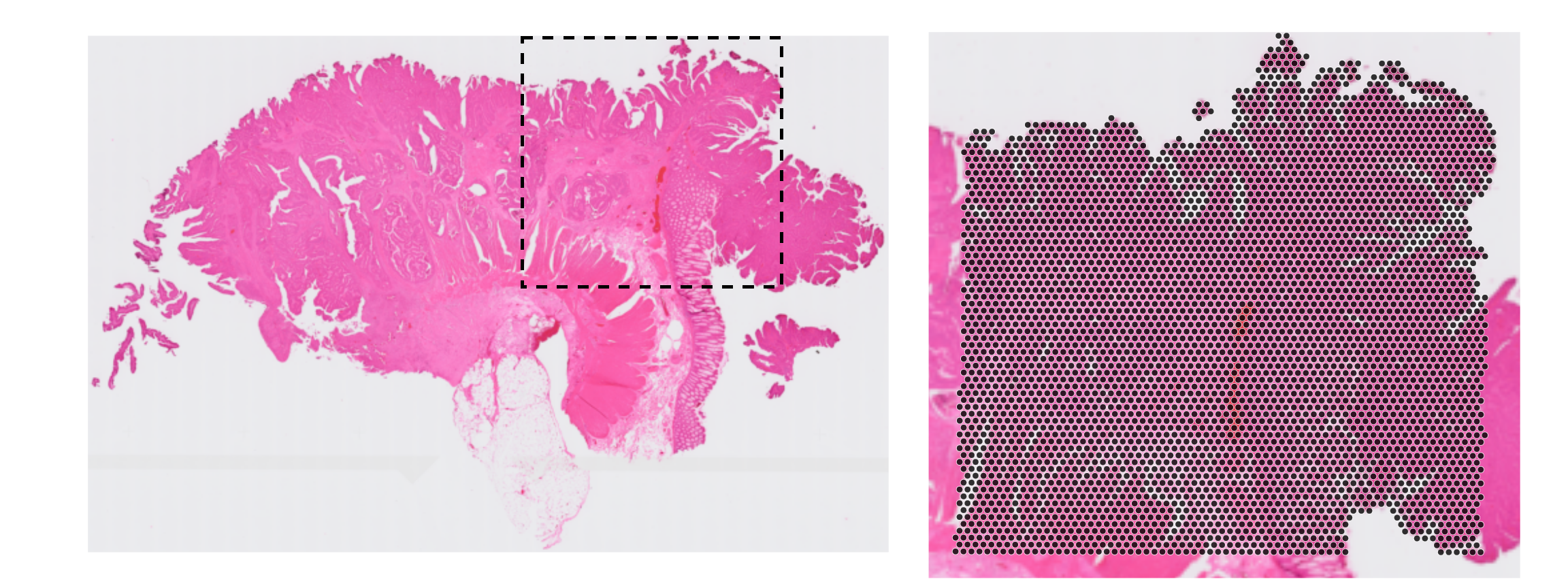
In this demo, we will be analyzing Visium data on a human colorectal cancer biopsy from Oliveira et al. (2024) (Chapter 6). Rather than recapitulating all possible analyses, our goal is to highlight those that might be of particular interest in the context of these data.

12.1.2 Dependencies

Code

library(osfr)
library(scran)
library(scater)
library(igraph)
library(AUCell)
library(scuttle)
library(spacexr)
library(msigdbr)
library(VisiumIO)
library(jsonlite)
library(ggspavis)
library(pheatmap)
library(patchwork)
library(OSTA.data)
library(BiocParallel)
library(DropletUtils)
library(SpatialExperiment)
# specify whether/how to 
# perform parallelization
bp <- MulticoreParam(th <- 10)
# set seed for random number generation
# in order to make results reproducible
set.seed(194849)

12.2 Data import

Code

# retrieve dataset from OSF repo
id <- "Visium_HumanColon_Oliveira"
pa <- OSTA.data_load(id)
dir.create(td <- tempfile())
unzip(pa, exdir=td)

Code

# read into 'SpatialExperiment'
obj <- TENxVisium(
    spacerangerOut=td, 
    format="h5", 
    images="lowres")
(spe <- import(obj))

##  class: SpatialExperiment 
##  dim: 18085 4269 
##  metadata(2): resources spatialList
##  assays(1): counts
##  rownames(18085): ENSG00000187634 ENSG00000188976 ... ENSG00000198695
##    ENSG00000198727
##  rowData names(3): ID Symbol Type
##  colnames(4269): AACAATGTGCTCCGAG-1 AACACCATTCGCATAC-1 ...
##    TGTTGGTGCGGAATCA-1 TGTTGGTGGACTCAGG-1
##  colData names(4): in_tissue array_row array_col sample_id
##  reducedDimNames(0):
##  mainExpName: Gene Expression
##  altExpNames(0):
##  spatialCoords names(2) : pxl_col_in_fullres pxl_row_in_fullres
##  imgData names(4): sample_id image_id data scaleFactor

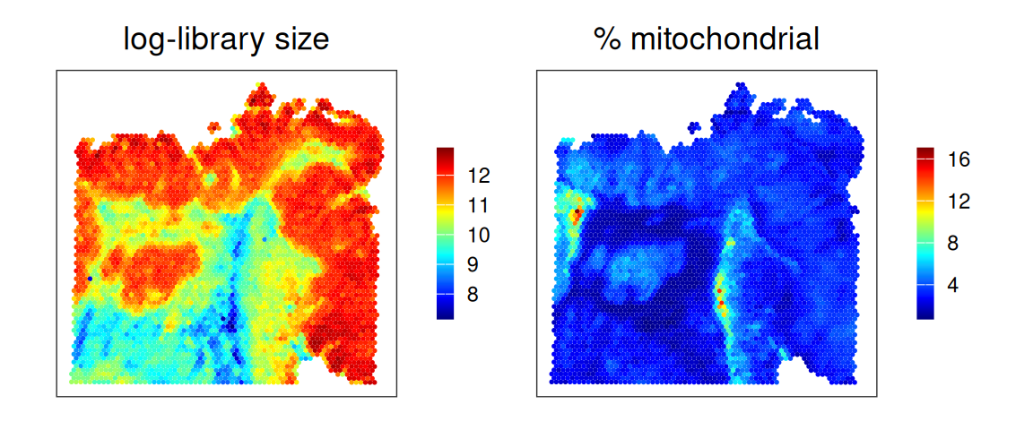
12.3 Quality control

Code

# use gene symbols as feature names
rownames(spe) <- make.unique(rowData(spe)$Symbol)
# add per-cell quality control metrics
sub <- list(mt=grep("^MT-", rownames(spe)))
spe <- addPerCellQCMetrics(spe, subsets=sub)

Code

# determine outliers via thresholding on MAD from the median
ol <- perCellQCFilters(spe, sub.fields="subsets_mt_percent")
# add results as cell metadata
colData(spe)[names(ol)] <- ol 
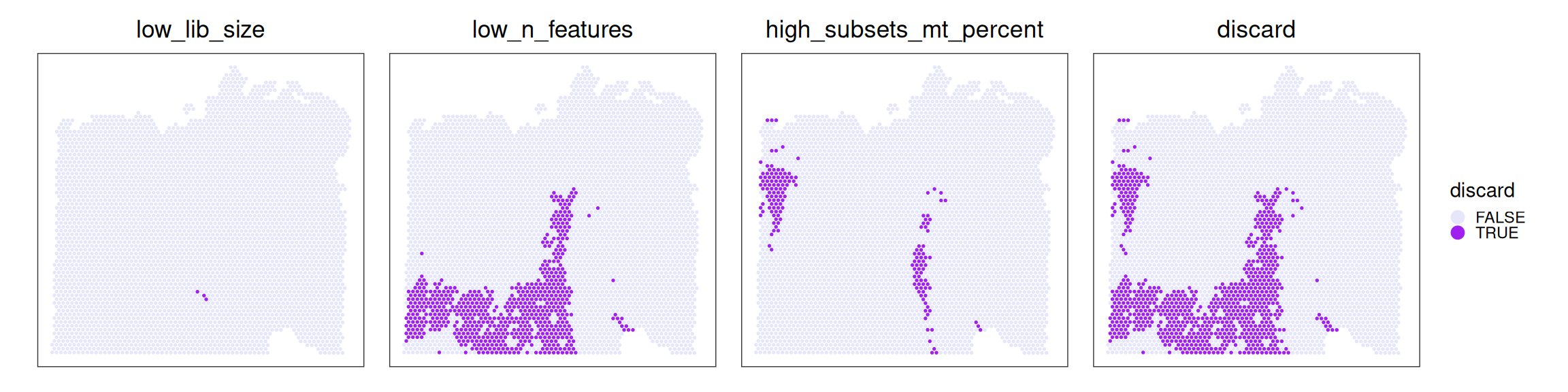
# tabulate # and % of cells that'd 
# be discarded for different reasons
data.frame(
    check.names=FALSE,
    `#`=apply(ol, 2, sum), 
    `%`=round(100*apply(ol, 2, mean), 2))

##                            #     %
##  low_lib_size              3  0.07
##  low_n_features          636 14.90
##  high_subsets_mt_percent 161  3.77
##  discard                 779 18.25

Let’s see which spots would be excluded according to the above criteria:

Code

lapply(names(ol), \(.) 
    plotSpots(spe, annotate=.) + ggtitle(.)) |>
    wrap_plots(nrow=1, guides="collect") &
    guides(col=guide_legend(override.aes=list(size=3))) &
    scale_color_manual("discard", values=c("lavender", "purple")) &
    theme(plot.title=element_text(hjust=0.5), legend.key.size=unit(0, "lines"))

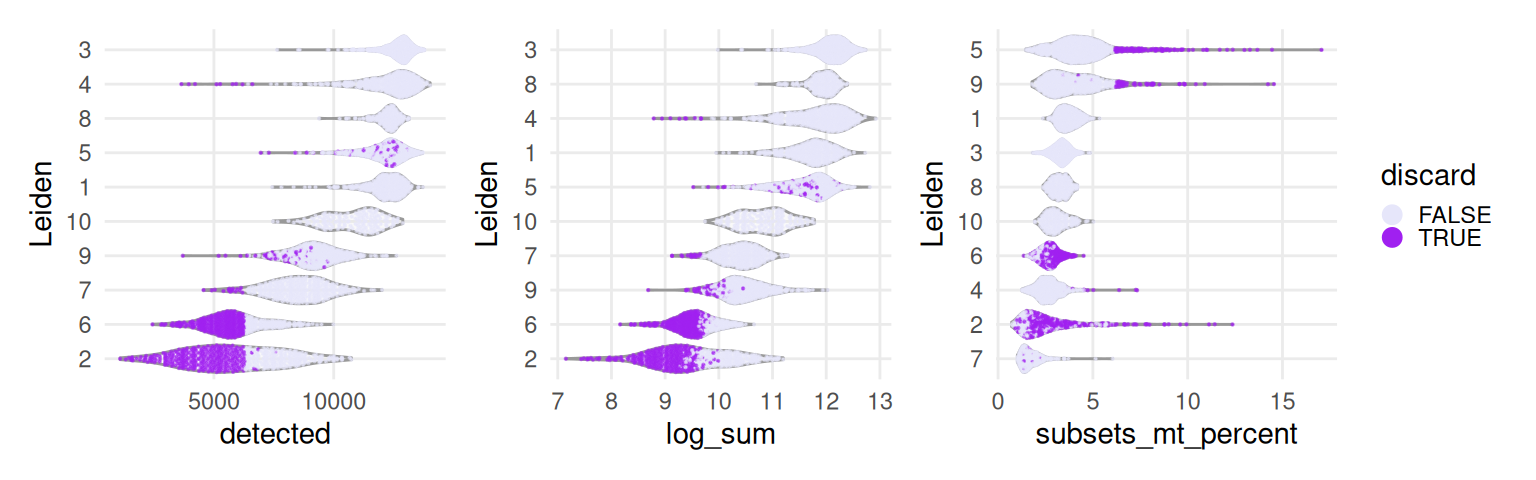
It seems like low-quality spots are highly spatially organized, so that might might decide to refrain from removing them, for now. We will see further below how the quality control metrics used here, and spots deemed to be discarded, are distributed across (transcription-based) clusters.

12.4 Processing

Code

# log-library size normalization
spe <- logNormCounts(spe)
# highly variable feature selection
tbl <- modelGeneVar(spe)
sel <- getTopHVGs(tbl, n=2e3)
# principal component analysis
spe <- runPCA(spe, subset_row=sel)

12.5 Clustering

As an unsupervised approach, we perform shared nearest-neighbor (SNN) graph-based clustering using the Leiden community detection algorithm.

Code

# build shared nearest-neighbor (SNN) graph
g <- buildSNNGraph(spe, use.dimred="PCA", type="jaccard")
# cluster via Leiden community detection algorithm
k <- cluster_leiden(g, objective_function="modularity", resolution=0.5)
table(spe$Leiden <- factor(k$membership))

##  
##    1   2   3   4   5   6   7   8   9  10 
##  326 504 710 432 732 458 315 171 469 152

12.6 Deconvolution

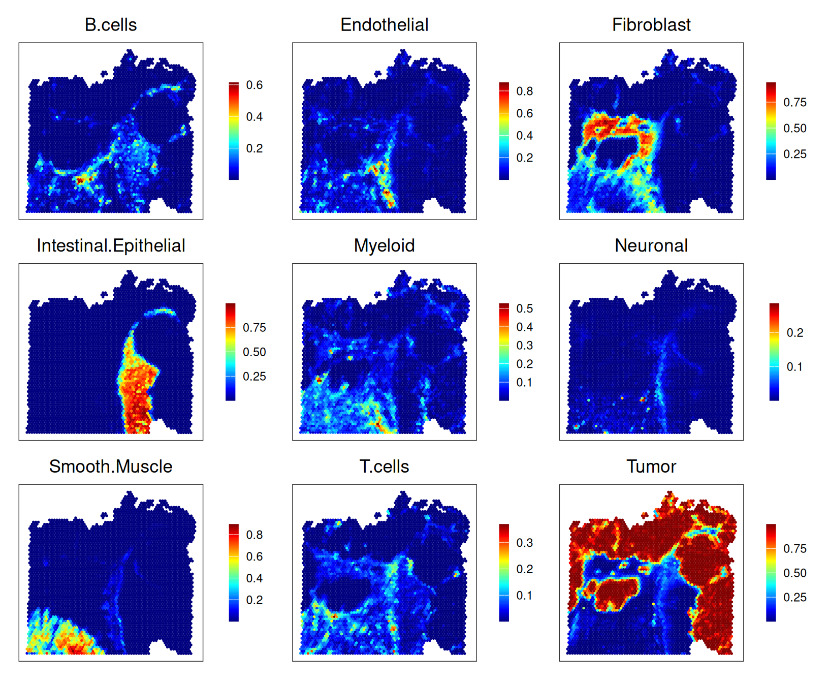
In a complementary approach, we deconvolute spot measurements using (annotated) reference single-cell data provided by the authors. Let’s first retrieve these data, alongside corresponding cell metadata, which includes low- (Level1) and high-resolution (Level2) annotations into 10 and 32 subpopulations, respectively.

Code

# retrieve dataset from OSF repo
id <- "Chromium_HumanColon_Oliveira"
pa <- OSTA.data_load(id)
dir.create(td <- tempfile())
unzip(pa, exdir=td)

Code

# read into 'SingleCellExperiment'
fs <- list.files(td, full.names=TRUE)
h5 <- grep("h5$", fs, value=TRUE)
sce <- read10xCounts(h5, col.names=TRUE)
# add cell metadata
csv <- grep("csv$", fs, value=TRUE)
cd <- read.csv(csv, row.names=1)
colData(sce)[names(cd)] <- cd[colnames(sce), ]
# use gene symbols as feature names
rownames(sce) <- make.unique(rowData(sce)$Symbol)
# exclude cells deemed to be of low-quality
sce <- sce[, sce$QCFilter == "Keep"]
# tabulate subpopulations
table(sce$Level1)

##  
##                B cells           Endothelial            Fibroblast 
##                  33611                  7969                 28653 
##  Intestinal Epithelial               Myeloid              Neuronal 
##                  22763                 25105                  4199 
##          Smooth Muscle               T cells                 Tumor 
##                  43308                 29272                 65626

Next, we perform deconvolution with spacexr (f.k.a. RCTD)(Cable et al. 2022). By default, runRctd()’s rctd_mode="doublet", i.e., at most two subpopulations are fit per pixel; here, we set rctd_mode="full" in order to allow for an arbitrary number of subpopulations to be fit instead.

Here, we filter the reference data to contain only cells from the same patient, and downsample to retain a limited number of cells per subpopulation. This is not strictly necessary, assuming that clusters are transcriptionally stable across patients, but helps with reducing runtime and memory consumption here.

Code

# prep reference data (Chromium);
# subset cells from same patient
.sce <- sce[, grepl("P2", sce$Patient)]
# downsample to at most 4,000 cells per cluster
cs <- split(seq_len(ncol(.sce)), .sce$Level1)
cs <- lapply(cs, \(.) sample(., min(length(.), 4e3)))
.sce <- .sce[, unlist(cs)]
# run 'RCTD' deconvolution
obj <- createRctd(spe, .sce, cell_type_col="Level1", max_cores=10)
(res <- runRctd(obj, rctd_mode="full"))

##  class: SpatialExperiment 
##  dim: 9 4269 
##  metadata(6): spatial_rna original_spatial_rna ... cell_type_info
##    internal_vars
##  assays(1): weights_full
##  rownames(9): B cells Endothelial ... T cells Tumor
##  rowData names(0):
##  colnames(4269): AACAATGTGCTCCGAG-1 AACACCATTCGCATAC-1 ...
##    TGTTGGTGCGGAATCA-1 TGTTGGTGGACTCAGG-1
##  colData names(1): sample_id
##  reducedDimNames(0):
##  mainExpName: NULL
##  altExpNames(0):
##  spatialCoords names(2) : x y
##  imgData names(0):

Weights inferred by RCDT should be normalized such that proportions of cell types sum to 1 in each spot:

Code

# scale weights such that they sum to 1
ws <- assay(res)
ws <- sweep(ws, 2, colSums(ws), `/`)
# add proportion estimates as metadata
ws <- data.frame(t(as.matrix(ws)))
colData(spe)[names(ws)] <- ws[colnames(spe), ]

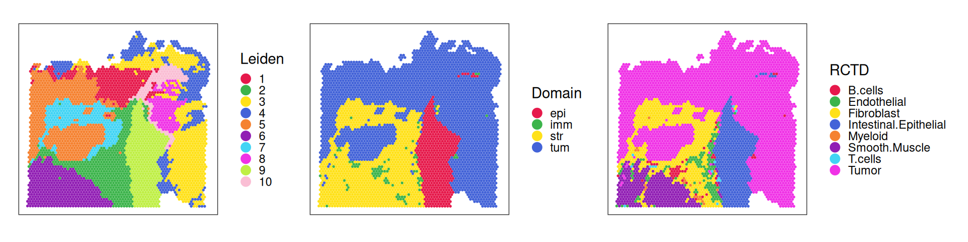
For comparison with unsupervised clustering (SNN-based Leiden), we also include assignments we would obtain if we were to assign spots the most frequent label (in terms of deconvolution estimates):

Code

ids <- names(ws)[apply(ws, 1, which.max)]
table(spe$RCTD <- factor(ids), spe$Leiden)

##                         
##                            1   2   3   4   5   6   7   8   9  10
##    B.cells                 0  42   0   6   0   4   0   0   0   0
##    Endothelial             0 113   0   0   0  23   0   0   0   0
##    Fibroblast              0 271   0   0  11  57 313   0   0   0
##    Intestinal.Epithelial   0   4   0   4   0   0   0   0 466  10
##    Myeloid                 0  16   0   0   2   3   0   0   0   0
##    Smooth.Muscle           0   8   0   0   0 362   0   0   0   0
##    T.cells                 0  11   0   0   0   3   0   0   0   0
##    Tumor                 326  39 710 422 719   6   2 171   3 142

We can also compartmentalize the tissue into broad biological compartments; here, by grouping RCTD-based subpopulation assignments into four classes:

Code

lab <- list(
    tum="Tumor",
    epi="Intestinal.Epithelial",
    imm=c("B.cells", "T.cells", "Myeloid"),
    str=c("Endothelial", "Fibroblast", "Smooth.Muscle"))
idx <- match(spe$RCTD, unlist(lab))
lab <- rep.int(names(lab), sapply(lab, length))
table(spe$Domain <- factor(lab[idx]))

##  
##   epi  imm  str  tum 
##   484   87 1158 2540

12.7 Exploratory

Let’s visualize deconvolution weights in space, i.e., coloring by the proportion of a given cell type estimated to fall within a given spot:

Code

lapply(names(ws), \(.) 
    plotSpots(spe, annotate=.)) |>
    wrap_plots(nrow=3) & theme(
    legend.key.width=unit(0.5, "lines"),
    legend.key.height=unit(1, "lines")) &
    scale_color_gradientn(colors=pals::jet())

Code

lapply(c("Leiden", "Domain", "RCTD"), 
    \(.) plotSpots(spe, annotate=.)) |>
    wrap_plots(nrow=1) &
    theme(legend.key.size=unit(0, "lines")) &
    scale_color_manual(values=unname(pals::trubetskoy()))

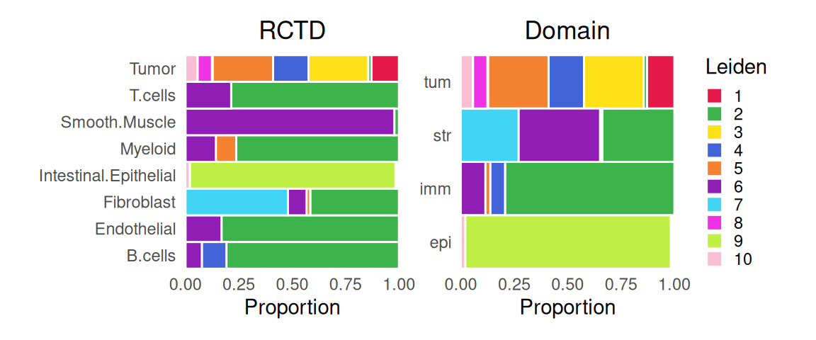
To help characterize subpopulations from unsupervised clustering, we can view their distribution across deconvolution-based clusters and broad domains; e.g., tumor spots are quite divers, while smooth muscle spots and (normal) epithelia map almost completely to a single cluster:

Code

cd <- data.frame(colData(spe))
df <- as.data.frame(with(cd, table(RCTD, Leiden)))
fd <- as.data.frame(with(cd, table(Domain, Leiden)))
ggplot(df, aes(Freq, RCTD, fill=Leiden)) + ggtitle("RCTD") +
ggplot(fd, aes(Freq, Domain, fill=Leiden)) + ggtitle("Domain") +
plot_layout(nrow=1, guides="collect") &
    labs(x="Proportion", y=NULL) &
    coord_cartesian(expand=FALSE) &
    geom_col(width=1, col="white", position="fill") &
    scale_fill_manual(values=unname(pals::trubetskoy())) &
    theme_minimal() & theme(aspect.ratio=1,
        legend.key.size=unit(2/3, "lines"),
        plot.title=element_text(hjust=0.5))

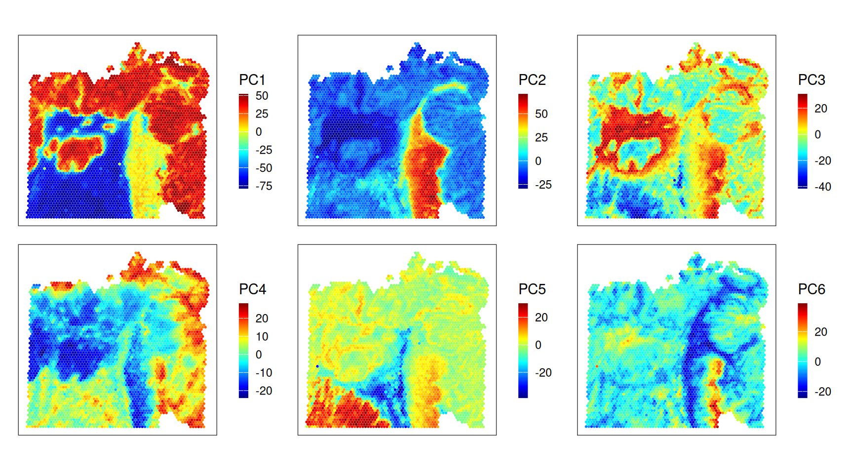
Let’s inspect the key drivers of (expression) variability in terms of PCs. Considering clustering and deconvolution results from above, we can see that

PC1 distinguishes stromal from both normal and malignant epithelia;
PC2 clearly separates (normal) intestinal epithelium from all else;
PC3 captures a fibroblast-rich region, and normal epithelia;
PC5 separates fibroblasts and smooth muscle cells; etc.

Code

pcs <- reducedDim(spe, "PCA")
colData(spe)[colnames(pcs)] <- pcs
lapply(colnames(pcs)[seq_len(6)], 
    \(.) plotSpots(spe, annotate=.) +
    scale_color_gradientn(., colors=pals::jet())) |>
    wrap_plots(nrow=2) & theme(
        plot.title=element_blank(),
        legend.key.width=unit(0.5, "lines"),
        legend.key.height=unit(1, "lines"))

Quality control metrics tend to be low for specific clusters. Their patch-like pattern, in turn, explains the clustering of low-quality spots seen earlier.

Code

lapply(c("detected", "log_sum", "subsets_mt_percent"), \(.)
    plotColData(spe, x=., y="Leiden", color_by="discard", point_size=0.1) +
    scale_x_discrete(limits=names(sort(by(spe[[.]], spe$Leiden, median))))) |>
    wrap_plots(nrow=1, guides="collect") &
    scale_color_manual("discard", values=c("lavender", "purple")) &
    guides(col=guide_legend(override.aes=list(alpha=1, size=3))) &
    theme_minimal() & theme(
        panel.grid.minor=element_blank(), 
        legend.key.size=unit(0, "lines"))

12.8 Signatures

Rather than investigating single genes, we can also evaluate the expression of sets of genes (e.g., pathway signatures); e.g., malignant tissue may differ in metabolic activity such as glycolysis and fatty acid metabolism, or exhibit increased apoptosis (cell death) etc. Here, we retrieve hallmark gene sets for some biological phenomena from MSigDB, using the msigdbr package:

Note that such gene lists like these may come from many different places - e.g., in-house analyses, other publications befitting the research question etc. As such, they may also be read into are from a .csv file, or stem from upstream analyses. In any case, they should be curated well and interpreted with caution.

Code

# retrieve hallmark gene sets from 'MSigDB'
db <- msigdbr(species="Homo sapiens", category="H")
# get list of gene symbols, one element per set
gs <- split(db$ensembl_gene, db$gs_name)
# simplify set identifiers (drop prefix, use lower case)
names(gs) <- tolower(gsub("HALLMARK_", "", names(gs)))
# how many sets?
length(gs)

##  [1] 50

Code

# how many genes in each?
range(sapply(gs, length))

##  [1]  34 335

Next, we will score these using AUCell (Aibar et al. 2017), which works in two steps: (i) rank genes for every observation (here, spots), and (ii) compute AUC values for each gene set. In essence, these represent the fraction of genes (within top-ranked genes; default 5%) that are in a given set; i.e., high values correspond to high activity (in terms of coordinated gene expression).

By definition, AUCell yields values in [0,1]. Larger sets (more genes) are more likely to achieve higher scores by chance (e.g., a gene set of all genes would score 1 in any dataset). It is thus unfair to compare them directly. However, spatial distribution, correlation, and relative comparisons between subpopulations etc. are still meaningful.

Code

# realize (sparse) gene expression matrix
mtx <- as(logcounts(spe), "dgCMatrix") 
# use ensembl identifiers as feature names
rownames(mtx) <- rowData(spe)$ID
# build per-spot gene rankings
rnk <- AUCell_buildRankings(mtx, BPPARAM=bp, plotStats=FALSE, verbose=FALSE)
# calculate AUC for each gene set in each spot
auc <- AUCell_calcAUC(geneSets=gs, rankings=rnk, nCores=th, verbose=FALSE)
# add results as spot metadata
colData(spe)[rownames(auc)] <- res <- t(assay(auc))

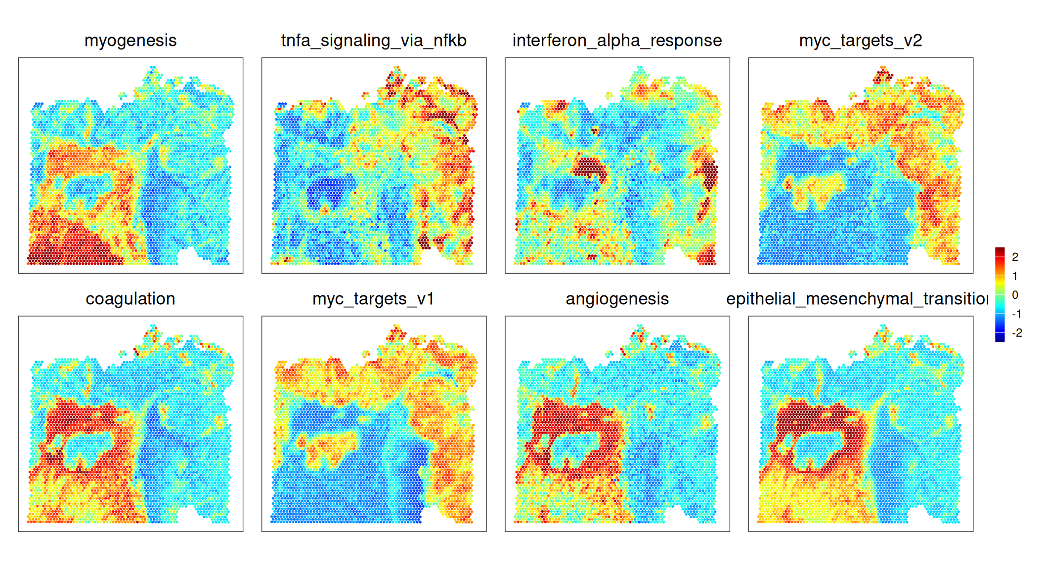
For simplicity, we’ll continue investigating only those signatures with the highest score variability across spots:

Code

var <- colVars(res) # variance across spots
top <- names(tail(sort(var), 8)) # top sets)

To summarize, MYC signalling is absent in stromal regions; the fibroblast ring surrounding a cancerous patch exhibits EMT, angiogenesis, etc.; INFa response and TNFa signalling is patch-like in both stroma and malignant epithelia.

Code

lapply(top, \(.) {
    spe[[.]] <- scale(spe[[.]]) # scaling
    plotSpots(spe, annotate=.) # plotting
}) |> 
    # arrange & prettify
    wrap_plots(nrow=2, guides="collect") & 
    scale_color_gradientn(
        colors=pals::jet(),
        oob=scales::squish, 
        limits=c(-2.5, 2.5)) & 
    theme(
        legend.key.width=unit(0.5, "lines"), 
        legend.key.height=unit(1, "lines"))

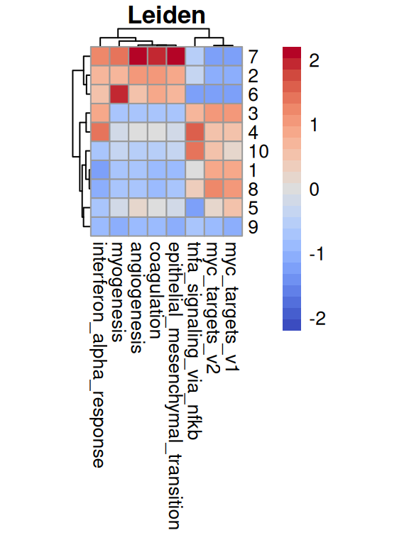
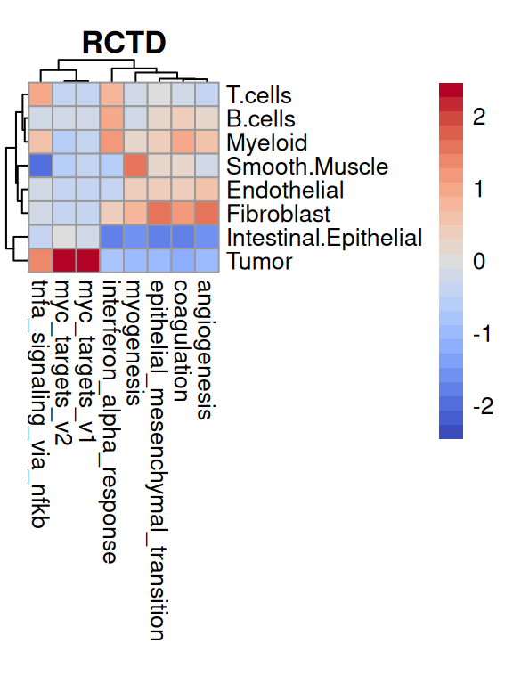
To ease interpretability, we can stratify AUCell scores by spot labels; these may stem from an unsupervised or deconvolution-based approach:

Code

for (. in c("Leiden", "RCTD")) {
    # aggregate AUC values by cluster
    mu <- aggregateAcrossCells(auc[top, ], spe[[.]], 
        use.assay.type="AUC", statistics="mean")
    # visualize as (cluster x set) heatmap
    pheatmap(
        mat=t(assay(mu)), scale="column", col=pals::coolwarm(), main=.,
        cellwidth=10, cellheight=10, treeheight_row=5, treeheight_col=5)
}

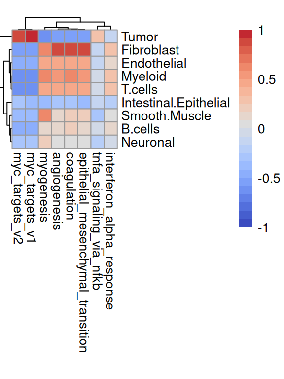
For the latter, we may instead correlate set scores with proportion estimates (rather than discretizing labels according to the dominant subpopulation):

Code

# correlate 'AUCell' signature scores with subpopulation
# proportion estimates from deconvolution with 'RCTD'
cm <- cor(as.matrix(ws), t(assay(auc[top, ])))

Code

pheatmap(cm, 
    col=pals::coolwarm(),
    breaks=seq(-1, 1, length=25),
    cellwidth=10, cellheight=10, 
    treeheight_row=5, treeheight_col=5)

12.9 Appendix

References

Aibar, Sara, Carmen Bravo González-Blas, Thomas Moerman, Vân Anh Huynh-Thu, Hana Imrichova, Gert Hulselmans, Florian Rambow, et al. 2017. “SCENIC: Single-Cell Regulatory Network Inference and Clustering.” Nature Methods 14 (11): 1083–86.

Cable, Dylan M., Evan Murray, Luli S. Zou, Aleksandrina Goeva, Evan Z. Macosko, Fei Chen, and Rafael A. Irizarry. 2022. “Robust Decomposition of Cell Type Mixtures in Spatial Transcriptomics.” Nature Biotechnology 40 (4): 517–26. https://doi.org/10.1038/s41587-021-00830-w.

Oliveira, Michelli F., Juan P. Romero, Meii Chung, Stephen Williams, Andrew D. Gottscho, Anushka Gupta, Susan E. Pilipauskas, et al. 2024. “Characterization of Immune Cell Populations in the Tumor Microenvironment of Colorectal Cancer Using High Definition Spatial Profiling.” bioRxiv. https://doi.org/10.1101/2024.06.04.597233.