Visium HD is a next-generation spatial transcriptomics technology developed by 10x Genomics, designed to provide single-cell resolution spatial gene expression data across entire tissue sections. Commercially available since 2024, Visium HD advanced the platform’s resolution from 55 µm spots to bins of subcellular resolution (2 µm). In this workflow, we will demonstrate common analysis steps with a Visium HD dataset on colorectal cancer (de Oliveira et al. 2025).
In this demo, we perform deconvolution on 16 µm bins and compare the concordance with results on 8 µm bins, provided by 10x Genomics.
Here, we only demonstrate the analysis for patient 2 (P2). Other patients, such as P1 and P5, also have public Chromium, Visium HD, and Xenium data available for the CRC group (see Chapter 6). It would be interesting to investigate the differences in malignant cells/bins (e.g., DEGs, pathways) between patients across different platforms.
Code
# retrieve dataset from OSF repoid<-"VisiumHD_HumanColon_Oliveira"pa<-OSTA.data_load(id)dir.create(td<-tempfile())unzip(pa, exdir=td)# read 8um bins into 'SpatialExperiment'vhd8<-TENxVisiumHD( spacerangerOut=td, processing="filtered", format="h5", images="lowres", bin_size="008")|>import()# use gene symbols as feature namesgs<-rowData(vhd8)$Symbolrownames(vhd8)<-make.unique(gs)vhd8
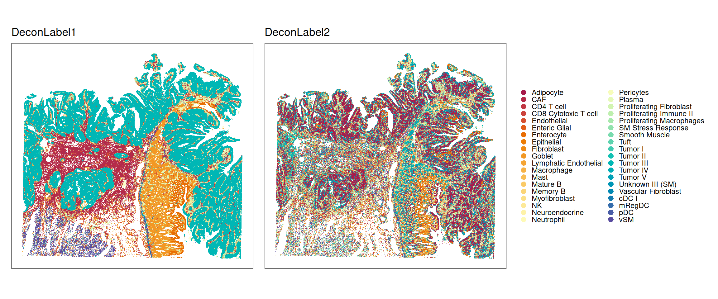
These data come with bin-level annotations from deconvolution estimates by RCTD(Cable et al. 2022), implemented in spacexr. Specifically, two sets of labels are available that correspond to the most and second most frequent of 38 cell types per bin, respectively:
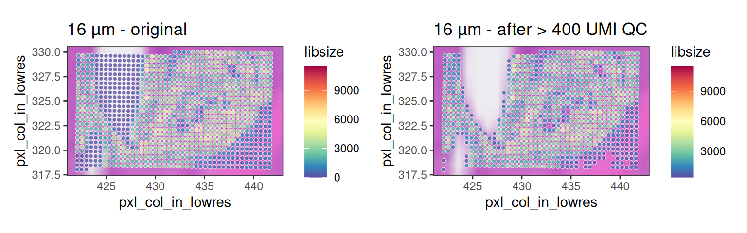
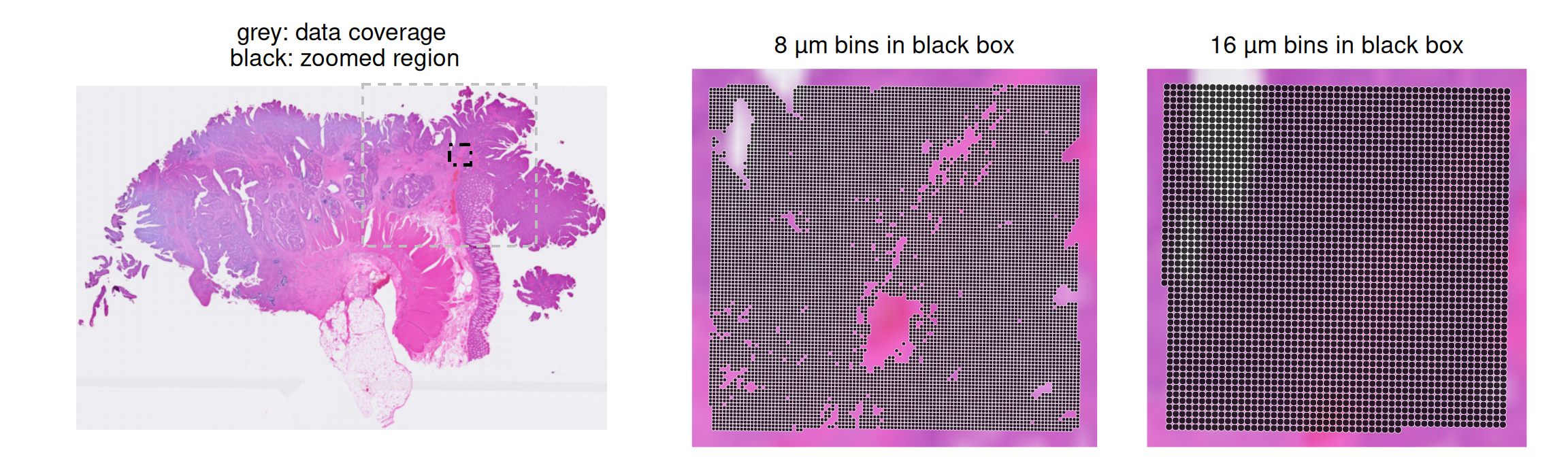
We can visualize such bins by zooming into an empty tissue region. On the left-hand side, one region shows a clear gap with low counts. Informed by H&E staining, bins located above tissue gaps should not be interpreted biologically, as the low counts in these bins are likely due to ambient RNA or transcript spillover. Therefore, they should be excluded from downstream analysis.
Based on a discussion with the original author at 10x Genomics, in this dataset, 8 µm bins with a library size below 100 are removed. Since we expect a 4-fold increase in library size across all bins at 16 µm, we can set the filtering threshold to 400.
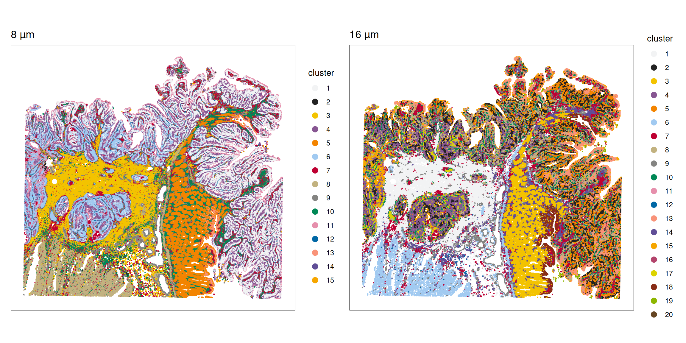
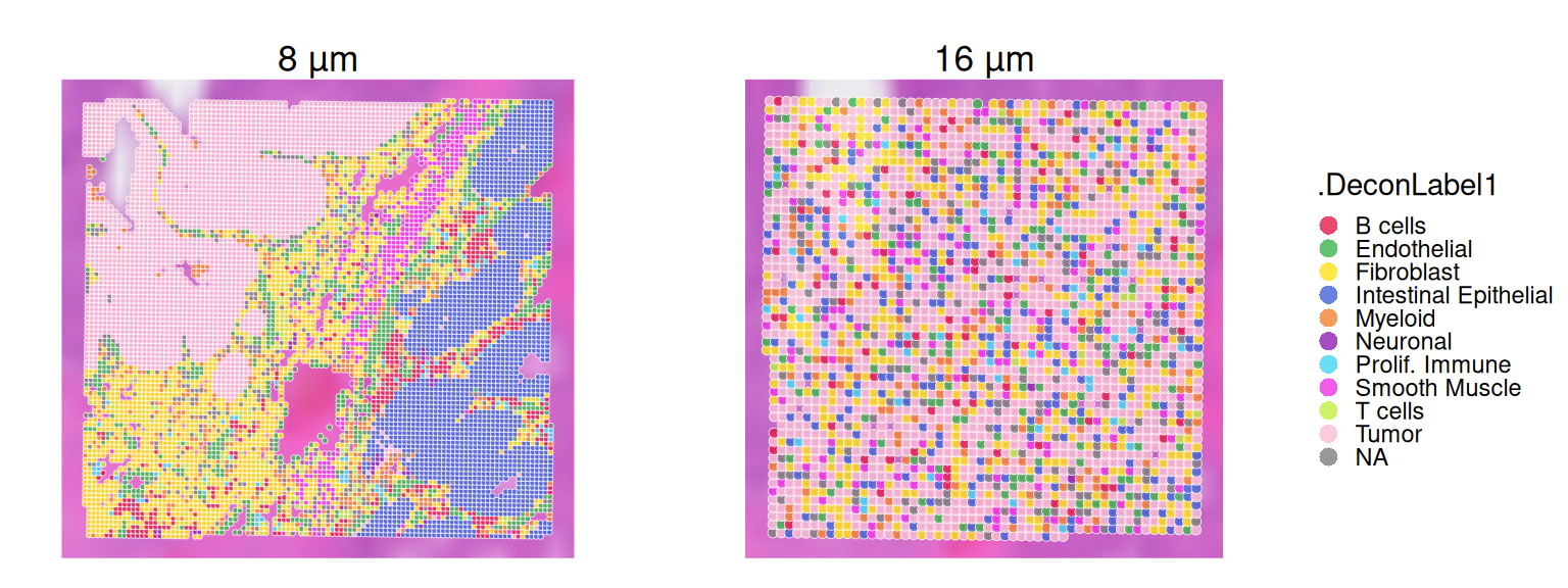
We can visualize the given clustering results at 8 µm and 16 µm resolutions. Later, we will compare the clustering result at 16 µm with that from Banksy.
To keep runtimes low, our downstream analysis will be performed on a subset area of 16 µm bins (1/64 of the data coverage area), which we read in here; there are no annotations available for this resolution in the public domain.
Note that 8 and 16 µm binned Visium HD data share the same full-resolution H&E image and scaling factor.
Code
.rng<- \(spe){xy<-spatialCoords(spe)*scaleFactors(spe)xs<-range(xy[, 1]); ys<-nrow(imgRaster(spe))-range(xy[, 2])x1<-xs[1]+4*(xs[2]-xs[1])/8; x2<-xs[2]-3*(xs[2]-xs[1])/8y1<-ys[1]+3*(ys[2]-ys[1])/8; y2<-ys[2]-4*(ys[2]-ys[1])/8list(box=c(x1, x2, y1, y2), cov=c(xs, ys))}vhd8r<-.rng(vhd8)# vhd16r <- .rng(vhd16) # use 8um bounding boxes to subset spes at both resolutions; # it is similar to 16um's box range .box<- \(roi, lty, lwd, col){geom_rect( xmin=vhd8r[[roi]][1], xmax=vhd8r[[roi]][2], ymin=vhd8r[[roi]][3], ymax=vhd8r[[roi]][4], col=col, fill=NA, linetype=lty, linewidth=lwd)}cov<-.box(roi="cov", lty=2, lwd=1/2, col="grey")box<-.box(roi="box", lty=4, lwd=2/3, col="black")# plotting.lim<- \(spe)list(xlim(spe[["box"]][c(1, 2)]),ylim(spe[["box"]][c(4, 3)]))plotVisium(vhd8, spots=FALSE, point_shape=22)+cov+box+ggtitle("grey: data coverage\n black: zoomed region")+plotVisium(vhd8, point_size=0.8, zoom=TRUE, point_shape=22)+.lim(vhd8r)+ggtitle("8 µm bins in black box")+plotVisium(vhd16, point_size=1.6, zoom=TRUE, point_shape=22)+.lim(vhd8r)+ggtitle("16 µm bins in black box")+plot_layout(nrow=1, widths=c(1.5, 1, 1))&facet_null()&theme(plot.title=element_text(hjust=0.5, vjust=0.5))
As detailed in Chapter 26, Banksy(Singhal et al. 2024) utilizes a pair of spatial kernels to capture gene expression variation, followed by dimension reduction and graph-based clustering to identify spatial domains.
Code
# set seed for random number generation# in order to make results reproducibleset.seed(112358)# 'Banksy' parameter settingsk<-8# consider first order neighborsl<-0.2# use little spatial informationa<-"logcounts"xy<-c("array_row", "array_col")# restrict to selected featurestmp<-.vhd16[hvg, ]# compute spatially aware 'Banksy' PCstmp<-computeBanksy(tmp, assay_name=a, coord_names=xy, k_geom=k)tmp<-runBanksyPCA(tmp, lambda=l, npcs=20)reducedDim(.vhd16, "PCA")<-reducedDim(tmp)## run UMAP (for visualization purposes only)# .vhd16 <- runUMAP(.vhd16, dimred="PCA")# build cellular shared nearest-neighbor (SNN) graphg<-buildSNNGraph(.vhd16, use.dimred="PCA", type="jaccard", k=20)# cluster using Leiden community detection algorithmk<-cluster_leiden(g, objective_function="modularity", resolution=1.2)table(.vhd16$Banksy<-factor(k$membership))
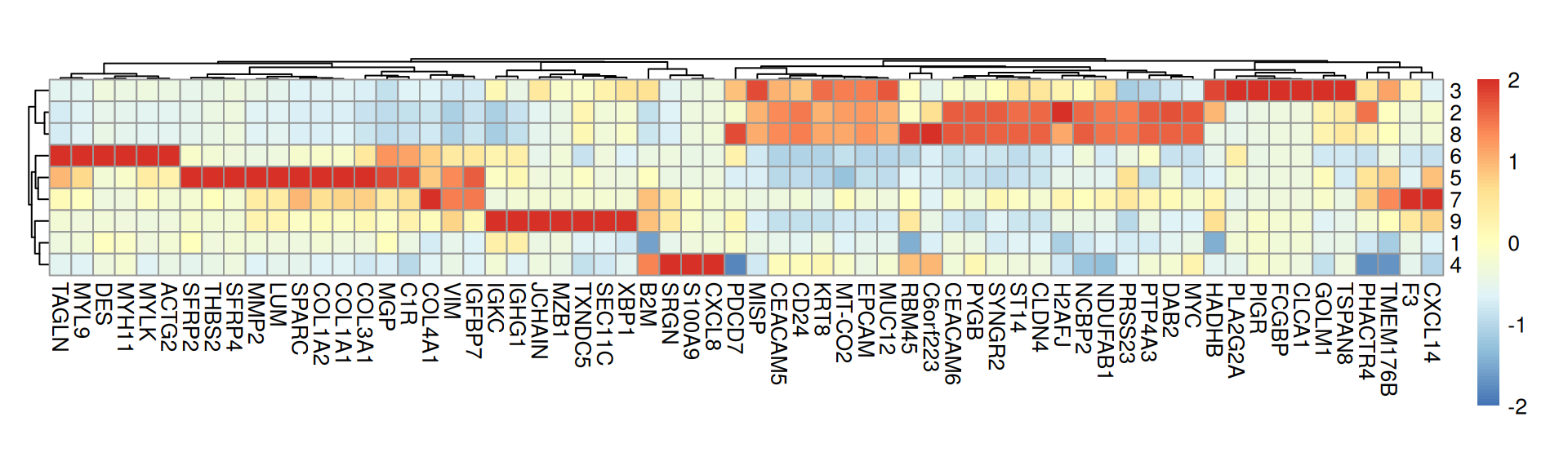
Next, we can perform differential gene expresison (DGE) analysis to identify markers for each cluster; c.f. Chapter 28. We also compute the cluster-wise mean expression of selected markers:
Code
# differential gene expression analysismgs<-findMarkers(.vhd16, groups=.vhd16$Banksy, direction="up")# select for a few markers per clustertop<-lapply(mgs, \(df)rownames(df)[df$Top<=2])top<-unique(unlist(top))# average expression by clusterspbs<-aggregateAcrossCells(.vhd16, ids=.vhd16$Banksy, subset.row=top, use.assay.type="logcounts", statistics="mean")
The marker genes in each cluster can be visualized with a heatmap:
We will now perform deconvolution on the 16 µm binned Visium HD data. First, we retrieve matching (Chromium) scRNA-seq data, which includes low- (Level1) and high-resolution (Level2) annotations of cells into 9 respectively 31 clusters. In order to ensure similar transcriptional profile across technologies, we filter the reference population to patient 2 only.
Code
# retrieve dataset from OSF repositoryid<-"Chromium_HumanColon_Oliveira"pa<-OSTA.data_load(id)dir.create(td<-tempfile())unzip(pa, exdir=td)# read into `SingleCellExperiment`fs<-list.files(td, full.names=TRUE)h5<-grep("h5$", fs, value=TRUE)sce<-read10xCounts(h5, col.names=TRUE)# add cell metadatacsv<-grep("csv$", fs, value=TRUE)cd<-read.csv(csv, row.names=1)colData(sce)[names(cd)]<-cd[colnames(sce), ]# use gene symbols as feature namesgs<-rowData(sce)$Symbolrownames(sce)<-make.unique(gs)# exclude cells deemed to be of low-qualitysce<-sce[, sce$QCFilter=="Keep"]# subset cells from same patientsce<-sce[, grepl("P2", sce$Patient)]sce
Note that "Proliferating Immune II" spans evenly between "B cells" and "Tumor", so we will make it a separate class, "Prolif. Immune" in the low-resolution annotations:
Below, these extra classes in the Visium HD 8 μm bin annotations will be ignored.
15.5.2 Simplify 8 µm annotations
We can merge the provided deconvolution annotation "DeconLabel1" (most likely cell type for singlets, most dominant type for doublets) into a lower resolution using the single-cell reference annotations:
Let us check the top-5 common doublet pairs according to the "doublet_certain" class:
Code
dbl<-vhd8$DeconClass=="doublet_certain"lab<-c(".DeconLabel1", ".DeconLabel2")df<-data.frame(colData(vhd8)[dbl, lab])# sort as to ignore orderdf<-apply(df, 1, sort)df<-do.call(rbind, df)names(df)<-lab# count unique pairsij<-paste(df[, 1], df[, 2], sep=";")head(sort(table(ij), decreasing=TRUE), 5)
##  ij
##       Myeloid;Tumor B cells;Fibroblast Fibroblast;Myeloid        Tumor;Tumor
##                3799               3670               3453               2742
##    Fibroblast;Tumor
##                2532
We can see that myeloid are commonly co-localized with tumor and fibroblasts cells; most doublets are homotypic, i.e., they are (mostly) composed of one low-resolution type.
Subset 8um bins within black bounding box
We can perform the same subsetting procedure to 8 µm bins and compare the difference in the number of bins in the zoomed (black box) area.
Code
# subset zoomed (black box) area.vhd8<-.sub(spe=vhd8, rng=vhd8r)# compare number of bins between resolutions(n<-ncol(.vhd8))
As expected, the number of 8 µm bins is about 4 times the number of 16 µm bins. We will visualize the same subset for both bin sizes in any downstream analyses.
15.5.3 Run RCTD on 16 µm bins
We also assume there are at most two cell types in a 16 µm bin as in 8 µm, and thus we would expect a smaller proportion of singlets.
Code
# downsample to at most 4,000 cells per cluster for 'sce'# (this is done only to keep runtime/memory low)cs<-split(seq_len(ncol(sce)), sce$Level1)cs<-lapply(cs, \(.)sample(., min(length(.), 4e3)))ncol(.sce<-sce[, unlist(cs)])rctd_data<-createRctd(.vhd16, .sce, cell_type_col="Level1")(res<-runRctd(rctd_data, max_cores=4, rctd_mode="doublet"))
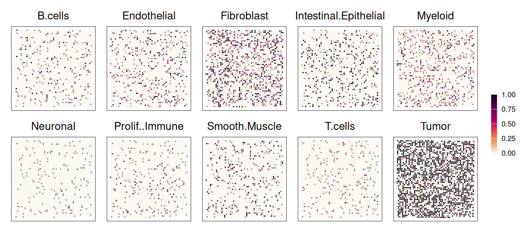
Weights inferred by RCTD correspond to proportions of cell types, such that they sum to 1 for a given observation (expect for rejected ones, which sum to 0):
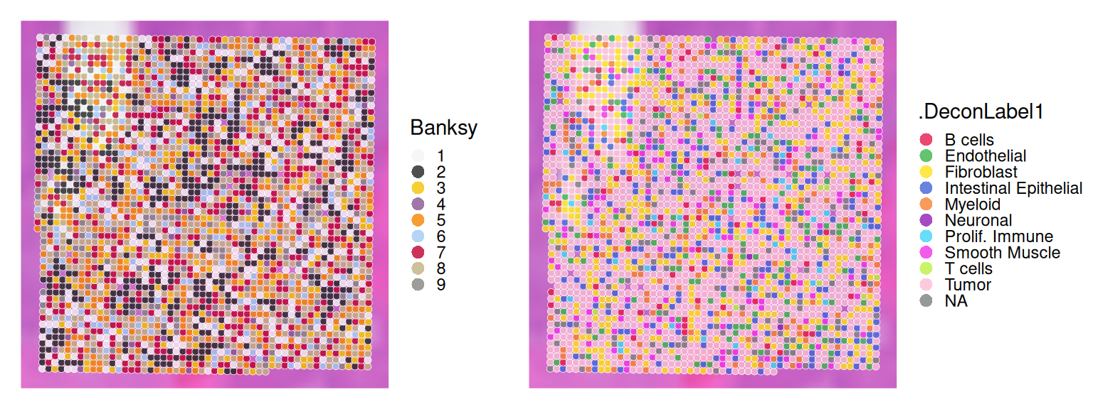
We observe clear agreement in deconvolution at both 8 µm and 16 µm resolutions; however, the 8 µm resolution better captures fine structures, such as the string-like shape of endothelial and fibroblast bins extending into the upper left tumor region.
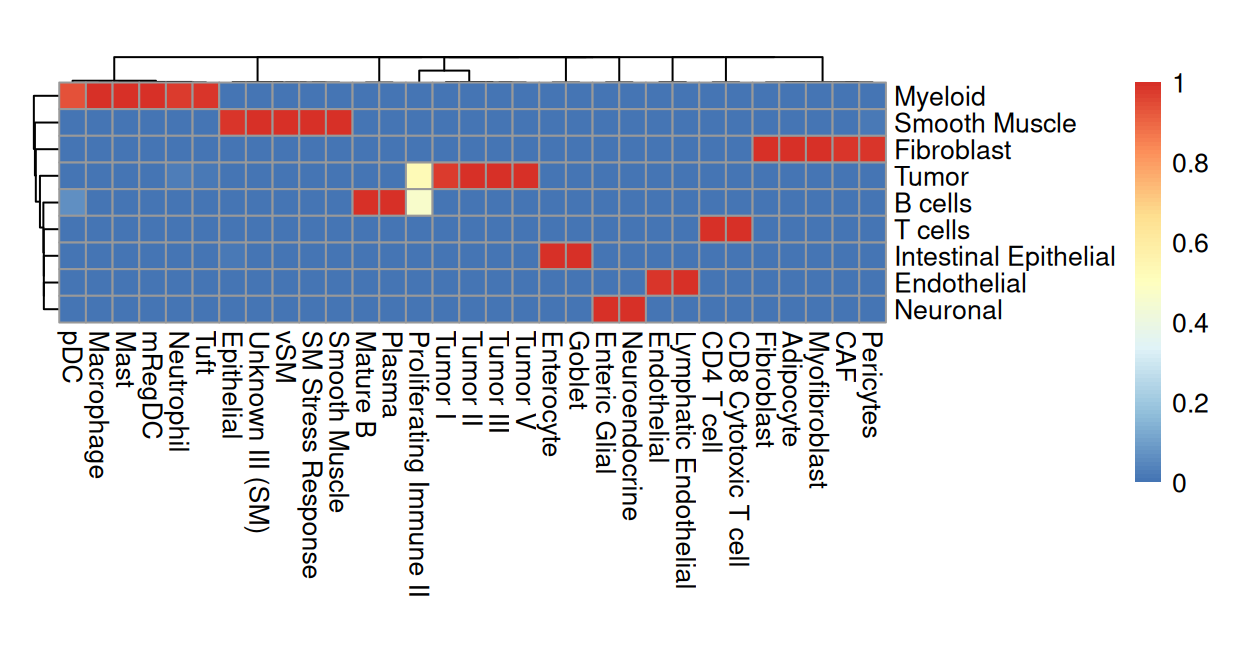
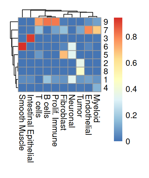
We observe that Banksy delineates tissue borders very well, while deconvolution provides direct biological insight into the underlying clusters. Their concordance can be visualized using a heatmap:
From the above heatmap, cluster 5 and 7 are mostly immune cells; cluster 9 maps to endothelial; cluster 1 and 13 correspond to intestinal epithelial and smooth muscle cells, respectively; fibroblasts map to cluster 10; tumor spans clusters 3, 11 and 12.
15.7 Neighborhood analysis
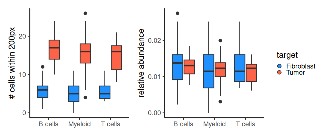
Here, we want to quantify the abundance between T cells, B cells, or Myeloid bins to Fibroblast or Tumor bins in 8 µm zoomed region. We use getAbundances() from Statial(Ameen et al. 2024) to calculate, for each bin, the abundance of other cell types within a radius of 200 px; the resulting (bins \(\times\) types) matrix is stored as reducedDim slot "abundances".
Now, we filter to only T cells, B cells and Myeloid bins, and investigate – within their neighborhood – the spatial proximity differences to Fibroblast or Tumor bins in terms of abundance.
##  # A tibble: 6 × 3
##    CT      target         n
##    <chr>   <chr>      <int>
##  1 Myeloid Tumor          0
##  2 Myeloid Fibroblast    43
##  3 B cells Tumor          0
##  4 B cells Fibroblast    50
##  5 B cells Tumor          0
##  6 B cells Fibroblast    50
In this region, we observe more fibroblast than tumor bins around each of the immune bins. However, note that in this zoomed region, we have nearly 1.4 times more fibroblast bins compared to tumor bins. Thus, we need to scale abundance values by the number of target cell type bins observed in the region.
After correction, we see amplified differences in the relative abundance of fibroblast bins compared to tumor bins around each immune cell type in the zoomed region.
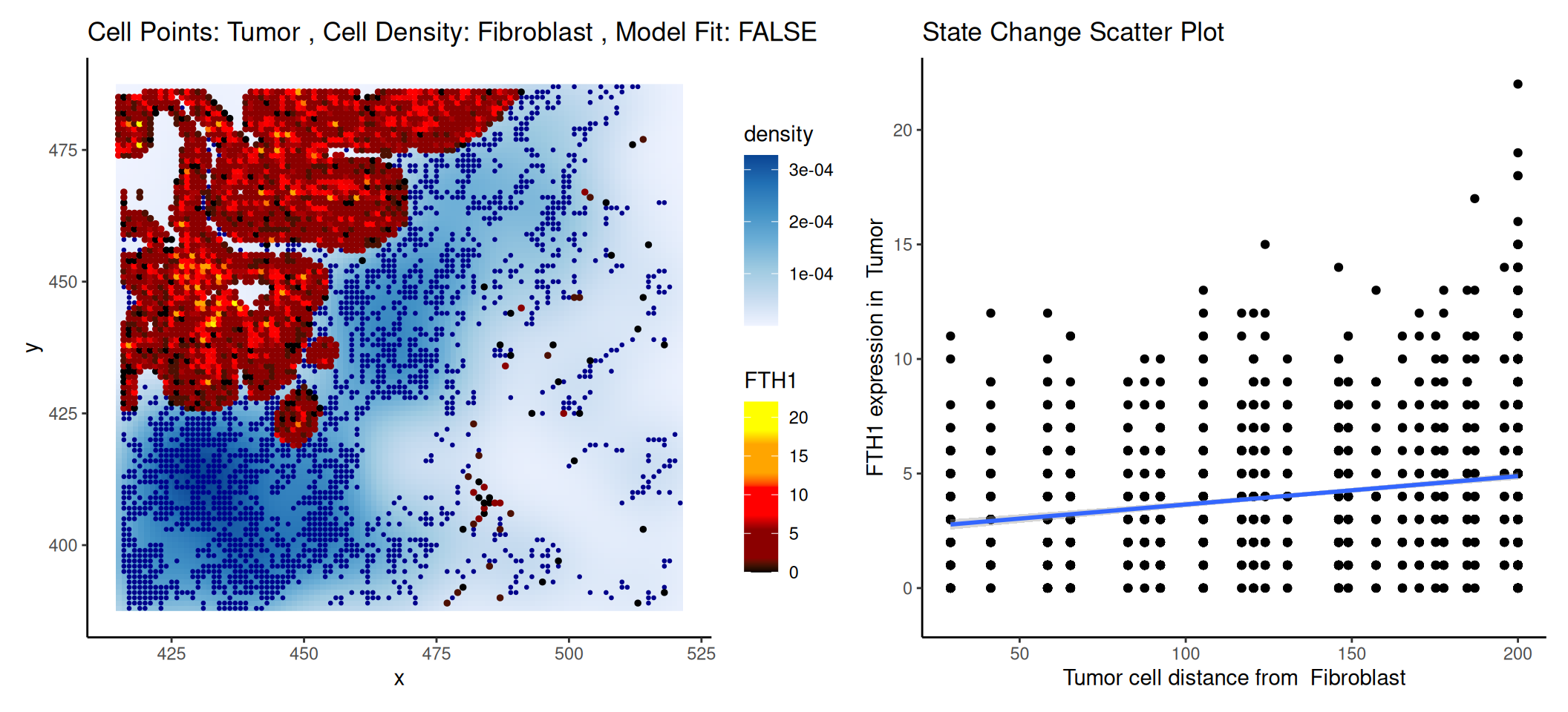
We can also investigate the “cell-cell-marker” relationship based on the minimum distance between two cell types within a given radius. The matrix of minimum distance between all pairwise cell types is stored in the reduced dimension, similar to how the abundance matrix was previously stored.
Code
# NOTE: conversion to SCE is a temporary fix for a 'Statial' bug # reported here: https://github.com/SydneyBioX/Statial/issues/16tmp<-as(.vhd8, "SingleCellExperiment")tmp<-getDistances(tmp, cellType=".DeconLabel1", imageID="sample_id", spatialCoords=names(xy), maxDist=200, nCores=4)reducedDim(.vhd8, "distances")<-reducedDim(tmp, "distances")
Here, we aim to determine whether the expression level of the tumor marker changes in proximity to fibroblast. Using FTH1 as an example, we observe a decrease in FTH1 expression in tumor bins as the distance to fibroblast increase. This trend could be visualized using a scatter plot.
The same analysis steps could be applied to the (unfiltered) 16 μm resolution data with the corresponding deconvolution results.
15.8 Conclusion
In this workflow, we demonstrated how to perform a standard analysis pipeline on a subset of Visium HD data binned at 16 µm. Most methods and visualization techniques developed for Visium can be applied to Visium HD. However, more sparsity is expected, as each data point (e.g. 2, 8, or 16 µm) has smaller area compared to Visium (55 µm). Each bin cannot be interpreted as a cell, but rather, a segmentation-free approach is applied here. Below are some resources for Visium HD to consider and incorporate into your pipeline:
Please see the following section for some cell-level Visium HD analysis guide.
Analysis pipeline by 10x Genomics (April 2024). The analysis consists of three steps: run StarDist nuclei segmentation in Python, sum gene expression into nuclei based on segmentation mask, and downstream analysis with scanpy and anndata.
Pipeline on cell typing for Visium HD in Python by Sanofi.
15.9 Cell-level Visium HD analysis
As of June, 2025, Visium HD enables direct output of H&E-segmented cell-level data, in addition to the previous binned_outputs at 2, 8, and 16 µm, from SpaceRanger v4. This update simplifies the additional cell segmentation required when using bin2cell or StarDist. However, a comparative study of segmentation methods on Visium HD data has yet to be conducted.
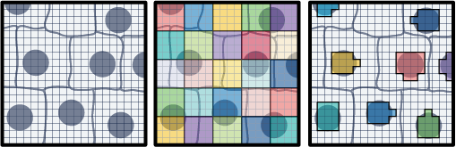
The morphology-driven, nucleus-based segmentation produces polygons representing nuclei and cells across the entire tissue, as illustrated in the schematics provided by 10x Genomics.
Figure 15.1: Two approaches for binning the 2x2 µm barcode squares in Visium HD data
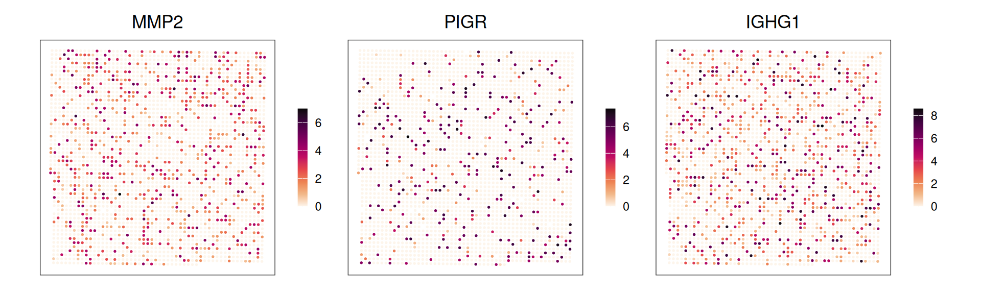
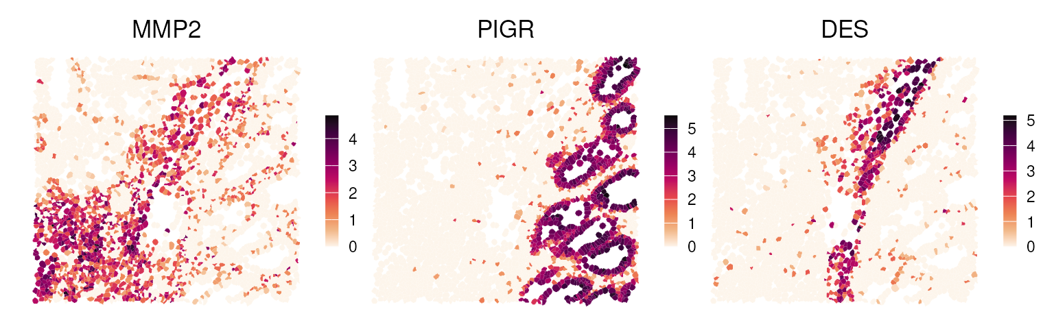
Compared to binned analysis, Visium HD with cell-level segmentation is more similar to Xenium data, but with full-transcriptome coverage. Most analytical methods are transferable; however, at single-cell resolution, deconvolving each data point into multiple cell types should be adapted using label transfer or unsupervised clustering to assign single-cell type labels. For example, after clustering, we identified three differentially expressed genes:
Figure 15.2: Differential marker gene expressions spatially visualized as polygons
Ameen, Farhan, Nick Robertson, David M. Lin, Shila Ghazanfar, and Ellis Patrick. 2024. “Kontextual: Reframing Analysis of Spatial Omics Data Reveals Consistent Cell Relationships Across Images.”bioRxiv. https://doi.org/10.1101/2024.09.03.611109.
Cable, Dylan M., Evan Murray, Luli S. Zou, Aleksandrina Goeva, Evan Z. Macosko, Fei Chen, and Rafael A. Irizarry. 2022. “Robust Decomposition of Cell Type Mixtures in Spatial Transcriptomics.”Nature Biotechnology 40: 517–26. https://doi.org/10.1038/s41587-021-00830-w.
de Oliveira, Michelli Faria, Juan Pablo Romero, Meii Chung, Stephen R. Williams, Andrew D. Gottscho, Anushka Gupta, Susan E. Pilipauskas, et al. 2025. “High-Definition Spatial Transcriptomic Profiling of Immune Cell Populations in Colorectal Cancer.”Nature Genetics 57: 1512–23. https://doi.org/10.1038/s41588-025-02193-3.
Singhal, Vipul, Nigel Chou, Joseph Lee, Yifei Yue, Jinyue Liu, Wan Kee Chock, Li Lin, et al. 2024. “BANKSY Unifies Cell Typing and Tissue Domain Segmentation for Scalable Spatial Omics Data Analysis.”Nature Genetics 56: 431–41. https://doi.org/10.1038/s41588-024-01664-3.