39 Imputation
39.1 Preamble
39.1.1 Introduction
As was previously discussed, most commonly employed imaging-based ST assays can resolve 100s to 1000s of features. Meanwhile, non-spatially resolved single-cell assays are able to capture transcripts across 10,000 gene features. To allow estimating the expression of genes that may not be available in an ST assay, we would like to integrate spatially resolved data with scRNA-seq data using common features, in order to predict missing features using nearest-neighbor cells (i.e., transcriptionally similar cells).
39.1.2 Dependencies
39.2 Data import
The analyses demonstrated here will use 313-plex Xenium data (10x Genomics) of a human breast cancer biopsy section and the Chromium Single Cell Gene Expression Flex applied to FFPE tissues (scFFPE-Seq) assay with around 18,000 features (Janesick et al. 2023).
39.2.1 Xenium
Code
# retrieve spatial data
id <- "Xenium_HumanBreast1_Janesick"
pa <- OSTA.data_load(id, mol=FALSE)
dir.create(td <- tempfile())
unzip(pa, exdir=td)

# read into & set sample identifier
spe <- readXeniumSXE(td, addTx=FALSE)
spe$sample_id <- "Xenium"
dim(spe)
## [1] 313 16778039.2.2 Chromium
We now load the single cell FFPE RNA-Seq assay. To streamline the demonstration, we consolidate some of the cell type annotations provided by 10x Genomics (i.e., Annotation) into the scRNA-seq assay. The single-cell assay has 18,082 features, some of which are available in the Xenium assay as well.
Code
# retrieve single-cell data
id <- "Chromium_HumanBreast_Janesick"
pa <- OSTA.data_load(id)
dir.create(td <- tempfile())
unzip(pa, exdir=td)

# read into, set gene symbols & sample identifier
h5 <- file.path(td, "filtered_feature_bc_matrix.h5")
sce <- read10xCounts(h5, col.names=TRUE)
rownames(sce) <- make.unique(rowData(sce)$Symbol)
sce$sample_id <- "Chromium"

# retrieve cell type labels
fs <- list.files(td, full.names=TRUE)
csv <- grep("csv$", fs, value=TRUE)
cd <- read.csv(csv, row.names=1)
colData(sce)[names(cd)] <- cd[colnames(sce), ]
dim(sce)
## [1] 18082 3036539.3 Analysis
39.3.1 Integration
Considering an omics assay as a matrix of measurement values where rows/columns correspond to features/observations, there are three possible scenarios for integration (Argelaguet et al. 2021). Specifically, methods applicable to each type of integration strategy depend on the choice of anchors used or, otherwise put, the dimension along which to integrate.
Firstly, experiments may involve multiple (biological or technical) replicates, requiring horizontal integration across cells that share a common feature space. Secondly, multi-modal assays can simultaneously extract different types of features from a given cell. Integration must then be vertical, i.e., across features measured from the same cells. Thirdly, technological limitations may require measuring different modalities from separate groups of cells, in which case diagonal integration across both different cells and features is necessary.
Single-cell transcriptomics data analyses are most commonly faced with horizontal integration. Methods for this task have been benchmarked extensively (Tran et al. 2020; Chazarra-Gil et al. 2021; Luecken et al. 2022). While these span diverse types of approaches, they often share conceptually similar steps. For example, model-based methods explicitly fit the transcriptional effects of batch assignment, while graph-based methods separately link points within and between batches. harmony (Korsunsky et al. 2019), which we demonstrate here, first represents batches in PCA space, and uses maximum diversity clustering followed by linear mixture modeling to compute a corrected embedding.
To accomplish data transfer across cells of either two assays (scRNA-seq and imaging-based ST), we first need to find cells that are similar between the two datasets. To this end, we use the common genes of both assays to integrate both datasets into a joint embedding space. Here, the objective is to find the nearest scRNA-seq cell neighbors of each Xenium cell in the joint embedding space, assuming that these cells will have similar transcriptional profiles.
We can integrate them on a transcriptional level; here, using harmony (Korsunsky et al. 2019). To this end, we first consolidate the scRNA-seq and Xenium data into one object:
Code
# normalization
sfs <- (. <- spe$cell_area)/median(.)
spe <- normalizeRnaCounts.se(spe, size.factors=sfs)
sce <- normalizeRnaCounts.se(sce)

# concatenate objects
length(gs <- intersect(rownames(spe), rownames(sce)))
## [1] 307Code
cd <- intersect(names(colData(spe)), names(colData(sce)))
obj <- lapply(list(spe, sce), \(x) {
    y <- logcounts(x <- x[gs, ])
    y <- as(y, "dgCMatrix")
    SingleCellExperiment(
        assays=list(logcounts=y),
        colData=colData(x)[cd])
}) |> do.call(what=cbind)

# add single-cell annotations
lab <- match(colnames(obj), colnames(sce))
obj$Annotation <- sce$Annotation[lab]
We now filter out cells with too few counts, and then perform PC-based harmony integration:
Code
# filtering to keep cells with at
# least 10% of features detected
det <- colMeans(logcounts(obj) > 0)
obj <- obj[, det >= 0.1]

# principal component analysis
# (w/o additional feature selection)
obj <- runPca.se(obj,
    features=rownames(obj),
    output.name=".PCA")

# 'harmony' integration (keeping uncorrected PCs)
pcs <- RunHarmony(
    reducedDim(obj, ".PCA"),
    meta_data=obj$sample_id,
    ncores=2, verbose=FALSE)
reducedDim(obj, "PCA") <- pcs

# dimensionality reduction before/after
# integration (for visualization only)
obj <- runUmap.se(obj, num.threads=th,
    reddim.type=".PCA", output.name=".UMAP")
obj <- runUmap.se(obj, num.threads=th,
    reddim.type="PCA", output.name="UMAP")
Let us now visualize the embedding of both Xenium and scRNA-seq cells to assess the mixing of observations from both datasets. We also check if scRNA-seq cells are well-partitioned given their annotations:
Code
.obj <- obj[, obj$sample_id == "Chromium"]
plotUMAP(obj, colour_by="sample_id", point_size=0, dimred=".UMAP") + ggtitle("uncorrected") +
plotUMAP(obj, colour_by="sample_id", point_size=0) + ggtitle("corrected") +
plotUMAP(.obj, colour_by="Annotation", point_size=0) + ggtitle("Chromium") +
plot_layout(nrow=1, guides="collect") &
    guides(col=guide_legend(override.aes=list(alpha=1, size=2))) &
    theme_void() & theme(
        aspect.ratio=1,
        legend.key.size=unit(0, "pt"),
        plot.title=element_text(hjust=0.5))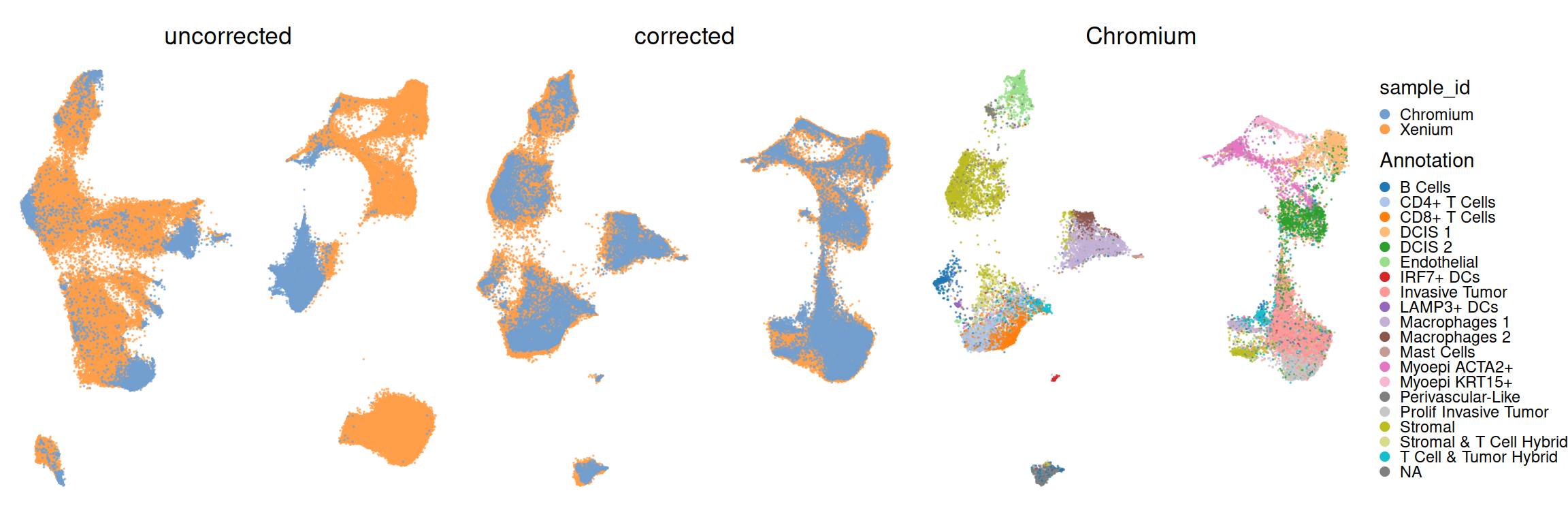
UMAPs like the one above are perhaps pretty, but not quantitative. We strongly encourage more quantitative metrics to quantify batch effects before and after correction, e.g., entropy, principal component regression, local inverse simpson index, silhouette width (problematic according to Rautenstrauch and Ohler (2025)), or similar. A number of such metrics have been proposed in benchmarks (see previous box), and many are implemented in CellMixS (Lütge et al. 2021).
Here, we will perform principal component regression (PCR) to quantify the variance explained by cluster/batch (before and after correction); after correction, we want most variation to be attributable to clusters.
Code
# helper to perform PCR
# xs = 'colData' to use as predictor(s)
# dr = 'reducedDim' slot to use as response
.pcr <- \(obj, xs, dr) {
    pcs <- reducedDim(obj, dr)
    lapply(xs, \(x) {
        fit <- summary(lm(pcs ~ obj[[x]]))
        r2 <- sapply(fit, \(.) .$adj.r.squared)
        data.frame(x, pc=seq_along(r2), r2)
    }) |> do.call(what=rbind)
}

# analysis
xs <- c("sample_id", "Annotation")
pcs <- list(before=".PCA", after="PCA")
pcr <- lapply(pcs, \(dr) .pcr(obj, xs, dr))

# wrangling
df <- bind_rows(pcr, .id="id")
df$id <- factor(df$id, names(pcs))
rownames(df) <- NULL
head(df)
## id x pc r2
## 1 before sample_id 1 0.005112371
## 2 before sample_id 2 0.032356284
## 3 before sample_id 3 0.023072209
## 4 before sample_id 4 0.031942048
## 5 before sample_id 5 0.140255895
## 6 before sample_id 6 0.001163737Visualizing coefficients of determination (R-squared), we can observe that batch effects were not that strong to begin with, and are virtually absent after correction; meanwhile, clusters explain similar amounts of variation before/after. This is interesting as the UMAPs visualized above would have suggested otherwise.
Code
# plot R2 before vs. after
ggplot(df, aes(pc, r2, col=x)) +
    facet_wrap(~id) +
    geom_line(show.legend=FALSE) + geom_point() +
    scale_x_continuous(breaks=c(1, seq(5, 20, 5))) +
    scale_y_continuous(limits=c(NA, 1), breaks=seq(0, 1, 0.2)) +
    labs(x="principal component", y="coeff. of determination") +
    guides(col=guide_legend("predictor", override.aes=list(size=2))) +
    coord_cartesian(xlim=c(1, 20)) +
    theme_bw() + theme(
        panel.grid.minor=element_blank(),
        legend.key.size=unit(0, "lines"))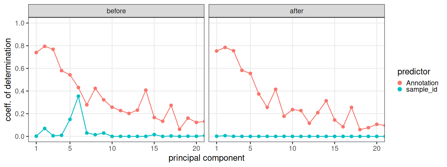
39.3.2 Selection
Here, we choose a small subset of features to transfer onto the Xenium assay. For this purpose, we test for differentially expressed genes (DEGs) between cell types (Annotation column), and select the top-20 markers for each:
Code
# test for differentially expressed genes
# (DEGs) to identify subpopulation markers
idx <- !is.na(sce$Annotation)
mgs <- scoreMarkers.se(
    sce[, idx], num.threads=th,
    groups=sce$Annotation[idx])

# get top markers per cell type
top <- lapply(names(mgs), \(k) {
    df <- mgs[[k]][c("mean", "detected", "auc.mean")]
    g <- head(rownames(df), 20)
    data.frame(k, g, df[g, ])
}) |> do.call(what=rbind)
rownames(top) <- NULL
head(top)
## k g mean detected auc.mean
## 1 B Cells MS4A1 2.934126 0.7587150 0.8733005
## 2 B Cells BANK1 1.787187 0.5748462 0.7811161
## 3 B Cells CD74 4.699715 0.9487355 0.7559122
## 4 B Cells CIITA 2.737434 0.7443609 0.7593737
## 5 B Cells CD79A 1.377933 0.5126452 0.7463857
## 6 B Cells TNFRSF13B 1.341701 0.4702666 0.730567439.3.3 Aggregation
Now that we have shown there is a correction for batch effects between Xenium and Chromium assays, we can transfer counts from single-cell onto Xenium data by identifying the k-nearest neighbors (kNNs) of each Xenium cell in the Chromium data, and imputing missing genes by aggregating their profile across kNNs (here, using mean expression).
Code
# find k-nearest neighbors across embeddings
# (from Xenium to Chromium cells)
idx <- split(colnames(obj), obj$sample_id)
pcs <- reducedDim(obj, "PCA")
ref <- pcs[idx$Chromium, ]
que <- pcs[idx$Xenium, ]
knn <- nn2(data=ref, query=que, k=k <- 20)

# create adjacency matrix
el <- cbind(
    rep(idx$Xenium, each=k),
    idx$Chromium[c(t(knn$nn.idx))])
g <- graph_from_edgelist(el, directed=TRUE)
A <- as_adjacency_matrix(g)

# average Chromium across Xenium neighbors
gs <- unique(top$g)
cs <- intersect(rownames(A), idx$Chromium)
ws <- A[idx$Xenium, cs]*(1/k)
y <- logcounts(sce)[gs, cs] %*% t(ws)
39.4 Downstream
39.4.1 Visualization
We now create two new SpatialExperiment objects by i) subsetting cells that passed our minimal filtering, and ii) replacing observed by imputed counts in one object:
Code
spe <- spe[, idx$Xenium]
spe <- normalizeRnaCounts.se(spe)
sqe <- SpatialExperiment(
    assays=list(logcounts=y),
    spatialCoords=spatialCoords(spe))
# needed for 'ggspavis' visualization
spe$in_tissue <- sqe$in_tissue <- 1
We can now compare imputed to observed counts. Here, we visualize ACTA2, which is included in both assays, as well as KRT17, which also marks myoepithelial cells:
Code
.p <- \(obj, col) {
    plotCoords(obj,
        point_size=0,
        annotate=col,
        assay_name="logcounts")
}
pal <- scale_color_gradient2("obs.", high="red")
qal <- scale_color_gradient2("imp.", high="blue")
.p(spe, "ACTA2") + pal +
.p(sqe, "ACTA2") + qal +
.p(sqe, "KRT17") + qal +
plot_layout(nrow=1) 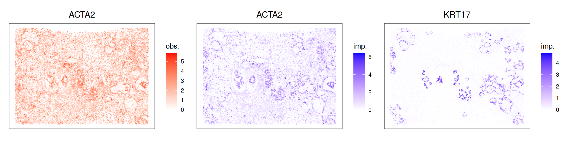
39.4.2 Comparison
As a more systematic comparison, we can visualize the correlation of cell-wise expression values (using shared features only) between observed and imputed data:
Code
gs <- intersect(rownames(spe), rownames(sqe))
imp <- as.matrix(t(logcounts(sqe[gs, ])))
obs <- as.matrix(t(logcounts(spe[gs, ])))
cm <- cor(imp, obs, method="pearson")
df <- data.frame(g=gs, p=diag(cm))
df$g <- factor(df$g, df$g[order(-df$p)])
ggplot(df, aes(g, p, fill=p > 0.5)) + geom_col() +
    labs(x="correlation (observed vs. imputed)", y=NULL) +
    geom_hline(yintercept=0.5) +
    theme_minimal() + theme(
        legend.position="none",
        panel.grid=element_blank(),
        axis.text.x=element_text(angle=90, vjust=0.5, hjust=1))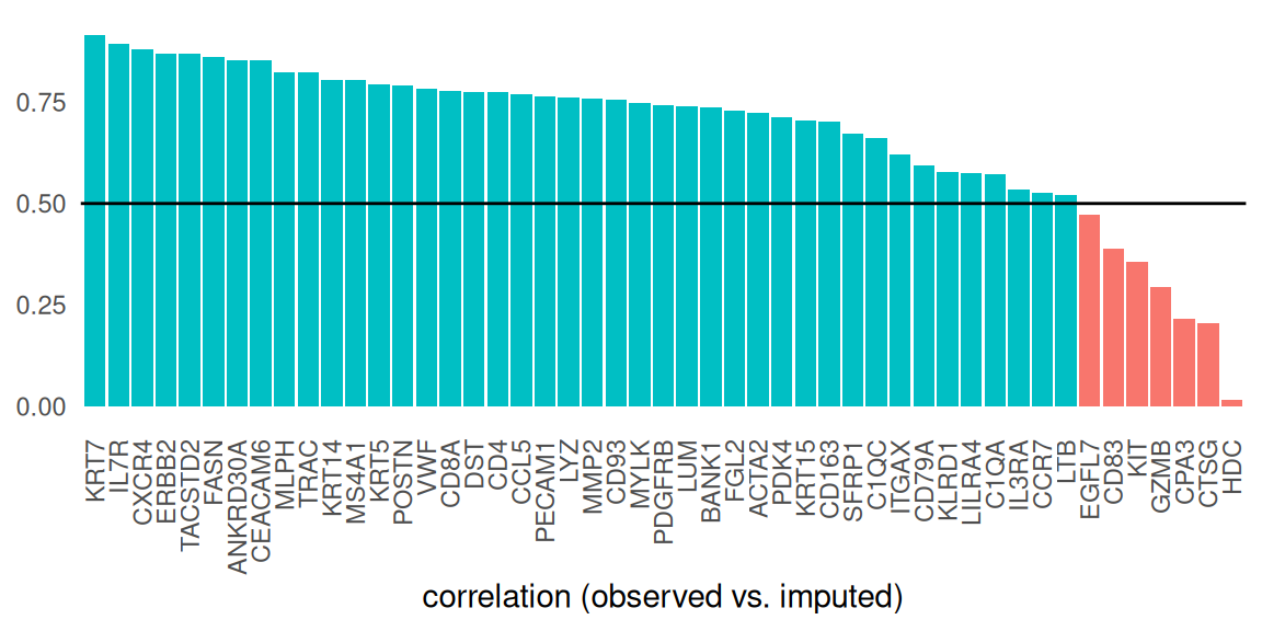
We observe the highest correlation between observed and imputed data for EPCAM; let’s confirm this by visualizing its expression in space:
Code
top <- levels(df$g)[1]
.p(spe, top) + pal +
.p(sqe, top) + qal +
plot_layout(nrow=1) 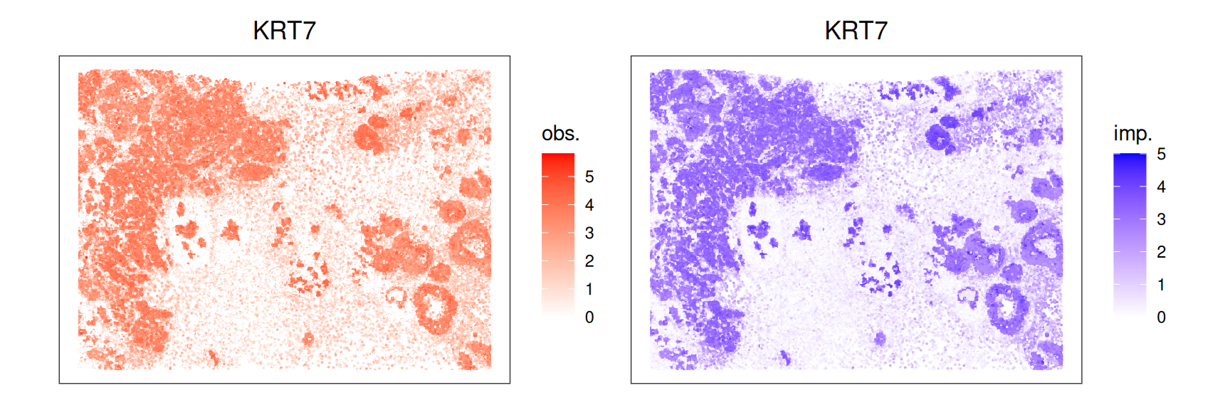
Genes that exhibit the lowest correlation tend to be rarely expressed. This arguably makes it difficult to identify similar Chromium cells and, in turn, accurately transfer information between both assays. By contrast, highly correlated genes are detected in a decent proportion of cells:
Code
##    GATA3    MLPH TACSTD2    IL7R    FASN   EPCAM
##     0.69    0.51    0.59    0.26    0.55    0.62
Code
fq(head(gs)) # low corr.## HDC CTSG CPA3 GZMB PLD4 CD83
## 0.32 0.01 0.03 0.08 0.03 0.0939.5 Other methods
Alternatively, we can use other R/Python frameworks to integrate imaging-based ST assays with scRNA-seq datasets, and impute missing features. Some of these methods could be used through R using packages such as reticulate and basilisk; see Chapter 8.
Tangram is available as a Python module through scvi-tools (Biancalani et al. 2021). The tool performs a softmax optimization to generate a probabilistic mapping between cells of scRNA-seq data and voxels (cells or spots) of ST data, which is then used to transfer labels or feature profiles across datasets.
LIGER is available in R via rliger (Welch et al. 2019), and incorporates a similar workflow performed in this chapter using harmony. The only difference between these approaches is how the joint embedding is obtained; here, LIGER uses non-negative matrix factorization (NMF). LIGER was originally proposed to perform this task for scRNA-seq and scATAC-seq assays.