22 Workflow: Xenium

22.1 Preamble

22.1.1 Introduction

In this demo, we will analyze 313-plex Xenium data on human breast cancer tissue (Janesick et al. 2023). Following very basic quality control and preprocessing, we will perform both (non-spatial) unsupervised clustering as well as fully supervised label-transfer based on scRNA-seq reference data; then compare the obtained cluster assignments to those provided by the authors.

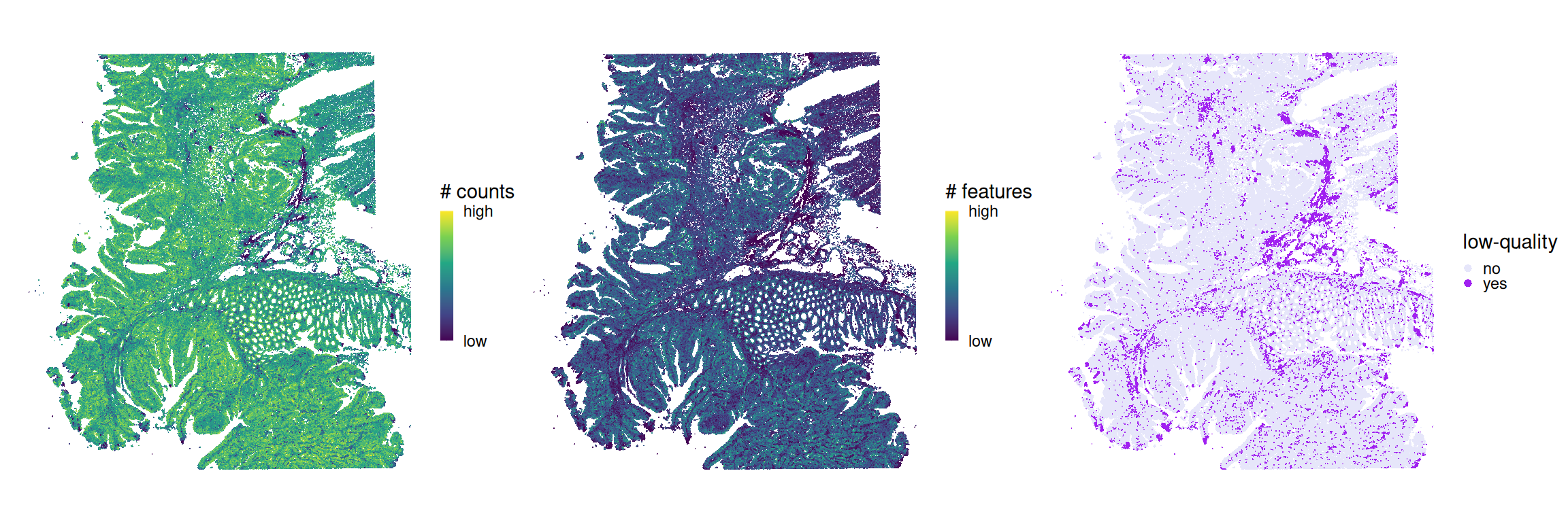
22.1.2 Dependencies

Code

library(dplyr)
library(tidyr)
library(scran)
library(igraph)
library(scater)
library(scuttle)
library(SingleR)
library(ggplot2)
library(patchwork)
library(OSTA.data)
library(BayesSpace)
library(BiocParallel)
library(DropletUtils)
library(SpatialExperiment)
library(SpatialExperimentIO)
# set parallelization
bp <- MulticoreParam(10)
# set seed for random number generation
# in order to make results reproducible
set.seed(112358)

Code

# retrieve dataset from OSF repository
id <- "Xenium_HumanColon_Oliveira"
pa <- OSTA.data_load(id)
dir.create(td <- tempfile())
unzip(pa, exdir=td)
(spe <- readXeniumSXE(td))

##  class: SpatialExperiment 
##  dim: 422 340837 
##  metadata(4): experiment.xenium transcripts cell_boundaries
##    nucleus_boundaries
##  assays(1): counts
##  rownames(422): ABCC8 ACP5 ... WFDC2 XCL2
##  rowData names(3): ID Symbol Type
##  colnames(340837): aaaadaba-1 aaaadgga-1 ... oikdmkkf-1 oikeebja-1
##  colData names(10): cell_id transcript_counts ... nucleus_area
##    sample_id
##  reducedDimNames(0):
##  mainExpName: NULL
##  altExpNames(3): NegControlProbe UnassignedCodeword
##    NegControlCodeword
##  spatialCoords names(2) : x_centroid y_centroid
##  imgData names(0):

Code

.plt_xy <- \(spe, col) {
    df <- data.frame(colData(spe), spatialCoords(spe))
    aes <- if (is.numeric(df[[col]])) {
        theme(
            legend.key.height=unit(1, "lines"), 
            legend.key.width=unit(0.5, "lines"))
    } else {
        list(
            theme(legend.key.size=unit(0, "lines")),
            guides(col=guide_legend(override.aes=list(alpha=1, size=2))))
    }
    ggplot(df, aes(x_centroid, y_centroid, col=.data[[col]])) +
        coord_equal() + theme_void() + aes +
        geom_point(stroke=0, size=1/3)
}

22.2 Quality control

Code

# compute cell-level QC metrics
spe <- addPerCellQCMetrics(spe)
# identify low-quality cells by thresholding on
# median absolute deviation (MAD) from the median
ol <- perCellQCFilters(spe)
# tabulate # and % of cells discarded 
# due to few counts/detected features
data.frame(
    check.names=FALSE,
    `#`=apply(ol, 2, sum), 
    `%`=round(100*apply(ol, 2, mean), 2))

##                     #    %
##  low_lib_size    8374 2.46
##  low_n_features 15313 4.49
##  discard        15313 4.49

Before proceeding to exclude any cells from downstream analyses, let’s first visualize the cells deemed to be of low quality in space alongside the underlying quality control metrics (total counts and detected features):

Code

spe$ol <- ol$discard
.plt_xy(spe, "sum") +  
    scale_color_viridis_c(
        "# counts", 
        trans="log1p",
        breaks=range(spe$sum), 
        labels=c("low", "high")) +
.plt_xy(spe, "detected") +
    scale_color_viridis_c(
        "# features", 
        breaks=range(spe$detected), 
        labels=c("low", "high")) +
.plt_xy(spe[, order(spe$ol)], "ol") + 
    scale_color_manual(
        "low-quality",
        labels=c("no", "yes"),
        values=c("lavender", "purple"))

Code

# discard low-quality cells
ncol(spe <- spe[, !ol$discard])

##  [1] 325524

22.3 Processing

For the sake of runtime, we will perform downstream analyses only on a square crop of the tissue, defined by the following px coordinates:

Code

box <- list(xmin=2e3, xmax=5e3, ymin=1e3, ymax=4e3)

Cropping to this region, we retain fewer than 90,000 cells:

Code

xy <- spatialCoords(spe)
i <- 
    xy[, 1] > box$xmin &
    xy[, 1] < box$xmax &
    xy[, 2] > box$ymin &
    xy[, 2] < box$ymax 
ncol(sub <- spe[, i])

##  [1] 88863

Code

df <- data.frame(xy, i)
p <- ggplot(df, 
    aes(x_centroid, y_centroid)) +
    coord_equal() + theme_void() + 
    theme(legend.position="none")
p + geom_point(aes(col=i), stroke=0, size=0.1) |
p + geom_point(data=df[i, ], stroke=0, size=0.2)

Next, we’ll log-normalize counts by area, and perform principal component analysis (PCA) on all 422 RNA targets:

Code

# cell area-based normalization
logcounts(sub) <- sweep(assay(sub), 2, sub$cell_area, `/`)
# principal component analysis
sub <- runPCA(sub, BPPARAM=bp)

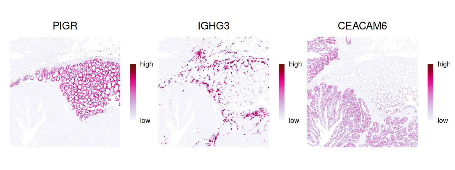
Let’s visualize the expression of some genes in space; e.g., PIGR, IGHG3 and CEACAM6, which should mark epithelial, plasma and tumor cells, respectively:

Code

gs <- c("PIGR", "IGHG3", "CEACAM6")
es <- scale(logcounts(sub))
es <- t(as.matrix(es[gs, ]))
colData(sub) <- cbind(colData(sub), es)
ps <- lapply(gs, \(.) .plt_xy(sub, .) + ggtitle(.))
wrap_plots(ps, nrow=1) &
    scale_color_gradientn(NULL, 
        labels=c("low", "high"), 
        colors=rev(hcl.colors(9, "PuRd")),
        limits=rng, breaks=rng <- range(es)) & 
    theme(plot.title=element_text(hjust=0.5))

22.4 Annotation

22.4.1 Unsupervised

Code

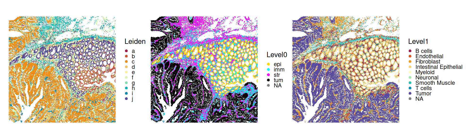
# shared nearest-neighbor (SNN) graph based on 
# cell-to-cell Jaccard similarity in PC space
g <- buildSNNGraph(sub, use.dimred="PCA", type="jaccard", BPPARAM=bp)
# community detection using Leiden algorithm
k <- cluster_leiden(g, objective_function="modularity", resolution=0.7)
table(sub$Leiden <- factor(. <- k$membership, labels=letters[seq_along(unique(.))]))

##  
##      a     b     c     d     e     f     g     h     i     j 
##   5855  3538 30354  4101  7646 11538  7404  3883  4705  9839

22.4.2 Supervised

For comparison, we annotate the Xenium data using a label transfer approach, SingleR, which relies on labeled scRNA-seq data to compute references profiles and transfers labels based on the rank correlation between observed (here, Xenium) and reference (scRNA-seq) expression profiles.

First, we retrieve a matching (Chromium) scRNA-seq dataset, which includes low- (Level1) and high-resolution (Level2) annotations of cells into 9 and 31 subpopulations, respectively:

Code

# retrieve dataset from OSF repository
id <- "Chromium_HumanColon_Oliveira"
pa <- OSTA.data_load(id)
dir.create(td <- tempfile())
unzip(pa, exdir=td)
# read into 'SingleCellExperiment'
sce <- read10xCounts(list.files(td, "h5$", full.names=TRUE))
cd <- read.csv(list.files(td, "cell_meta", full.names=TRUE))
colData(sce) <- cbind(colData(sce), cd[, -1])
table(sce$Level1) # tabulate low-res. labels
ncol(sce) # overall number of cells

##  
##                B cells           Endothelial            Fibroblast 
##                  33611                  7969                 28653 
##  Intestinal Epithelial               Myeloid              Neuronal 
##                  22763                 25105                  4199 
##            QC_Filtered         Smooth Muscle               T cells 
##                  19103                 43308                 29272 
##                  Tumor 
##                  65626 
##  [1] 279609

Here, we run SingleR using high-res. annotations (Level2) and with argument aggr.ref=TRUE, such that reference profiles will be aggregated (per cluster) prior to annotation. In this way, every single Xenium cell will be assigned a label based on which pseudo-bulk scRNA-seq profile represents the best match.

Note that we filter the reference data to contain only cells from the same patient. This is not strictly necessary, assuming that clusters are transcriptionally stable across patients, but is done here to reduce runtime.

Code

# exclude cells deemed to be of low-quality
sce <- sce[, sce$QCFilter == "Keep"]
# subset cells from same patient
sce <- sce[, grepl("P2", sce$Patient)]
# realize count matrix
assay(sce) <- as(assay(sce), "dgCMatrix")
# log-library size normalization
sce <- logNormCounts(sce)
# restrict to Xenium targets
sce <- sce[rowData(sce)$ID %in% rowData(sub)$ID, ]
# set gene symbols as feature names
rownames(sce) <- rowData(sce)$Symbol
# perform label transfer at the single cell-level,
# using pseudo-bulk Chromium profiles as reference
res <- SingleR(
    test=sub, ref=sce, 
    labels=sce$Level2, 
    aggr.ref=TRUE, BPPARAM=bp)
sub$Level2 <- factor(res$pruned.labels)

Based on these predictions, we can also propagate low-res. annotations (Level1):

Code

idx <- match(sub$Level2, sce$Level2)
table(sub$Level1 <- factor(sce$Level1[idx]))

##  
##                B cells           Endothelial            Fibroblast 
##                   6450                  4783                 10138 
##  Intestinal Epithelial               Myeloid              Neuronal 
##                  11888                  7206                   422 
##          Smooth Muscle               T cells                 Tumor 
##                   4250                  4998                 38373

Simplifying further, we can group cells into different compartments, namely, (malignant) tumor, immune, epithelial and stromal cells; we’ll see below that visualizing cells in this way nicely captures the general tissue structure.

Code

lab <- list(
    tum=c("Tumor"),
    epi=c("Intestinal Epithelial"),
    imm=c("B cells", "T cells", "Myeloid"),
    str=c("Endothelial", "Fibroblast", "Smooth Muscle"))
idx <- match(sub$Level1, unlist(lab))
lab <- rep.int(names(lab), sapply(lab, length))
table(sub$Level0 <- factor(lab[idx]))

##  
##    epi   imm   str   tum 
##  11888 18654 19171 38373

22.4.3 Comparison

Tabulating the cluster assignments between Leiden (unsupervised) and SingleR (supervised), we can observe overall high concordance; i.e., most clusters have a one-to-one mapping between both approaches. However, some subpopulations are split between clusters; e.g., cells labeled as cluster fibroblasts, endothelia and smooth muscle cells by SingleR tend to intermix in the Leiden clusters. This is not unexpected, given that these are all stromal subpopulations with comparatively similar transcriptional profiles. (Note that we are observing a mere fraction of the whole transcriptome with the Xenium panel employed here.)

Code

# contingency table & number of clusters
round(100*prop.table(table(sub$Level1, sub$Leiden), 2), 1)

##                         
##                             a    b    c    d    e    f    g    h    i    j
##    B cells                2.5  1.3  0.0  0.0 75.9  0.6  3.4  1.4  1.8  0.1
##    Endothelial            1.3  0.7  0.0  0.1  2.1 34.3  3.7  1.3  5.1  0.0
##    Fibroblast             6.2  5.8  0.0  0.1  5.9 50.9 14.9 46.5  6.7  0.4
##    Intestinal Epithelial  0.2 77.7  0.1  0.1  0.2  0.1  0.9  0.0  0.9 91.6
##    Myeloid                4.5  3.4  0.1  0.2  5.4  1.5 65.7  1.3 25.8  1.4
##    Neuronal               0.1  1.3  0.0  0.0  0.4  0.4  0.8  0.1  1.2  1.8
##    Smooth Muscle          2.1  6.0  0.0  0.0  2.3 10.3  5.3 46.3  6.5  0.7
##    T cells               69.1  2.1  0.0  0.1  2.8  0.8  2.9  2.6  3.9  0.8
##    Tumor                 14.2  1.6 99.8 99.3  4.9  1.2  2.5  0.4 48.1  3.3

Code

c(SingleR=nlevels(sub$Level1), Leiden=nlevels(sub$Leiden))

##  SingleR  Leiden 
##        9      10

Code

lapply(c("Leiden", "Level0", "Level1"), \(.) {
    pal <- if (. == "Level0") {
        c("gold", "cyan", "magenta", "black")
    } else {
        hcl.colors(nlevels(sub[[.]]), "Spectral")
    }
    .plt_xy(sub, .) + scale_color_manual(values=pal) 
}) |> wrap_plots()

22.5 Downstream

22.5.1 Marker genes

Below, we test for differential expression between Level1 clusters, and visualize selected markers as a heatmap of (z-scaled) average expression. It’s comforting to see that we pick up on many classics, e.g., endothelia are marked by VWF and PECAM1, T cells by CD2 and TRAC, etc.

Code

# test for differential expression between clusters
mgs <- findMarkers(sub, groups=sub$Level1, direction="up")
# select top-ranked genes for every cluster
top <- unique(unlist(lapply(mgs, \(df) rownames(df)[df$Top <= 3])))
plotGroupedHeatmap(sub, 
    features=top, group="Level1", 
    scale=TRUE, center=TRUE, fontsize=6)

References

Janesick, Amanda, Robert Shelansky, Andrew D. Gottscho, Florian Wagner, Stephen R. Williams, Morgane Rouault, Ghezal Beliakoff, et al. 2023. “High Resolution Mapping of the Tumor Microenvironment Using Integrated Single-Cell, Spatial and in Situ Analysis.” Nature Communications 14 (1): 8353.