31 Structure-based analysis

31.1 Preamble

31.1.1 Introduction

Spatial omics data further allow us to quantify various features that are related to tissue architecture. This allows us to perform comparisons of anatomical structure-derived features. We will refer to this type of analysis as structure-based analysis.

We will use the sosta package to reconstruct and quantify pancreatic islets from human donors suffering different stages of diabetic type 1 (T1D) and healthy controls (Damond et al. 2019). We will then compare some of the features between conditions.

31.1.2 Dependencies

Code

library(sosta)
library(ggplot2)
library(dplyr)
library(tidyr)
library(SpatialExperiment)
library(ExperimentHub)
library(lme4)
library(lmerTest)
library(ggfortify)
library(osfr)

Code

set.seed(8048)

31.1.3 Load data

We will load the data directly from ExperimentHub and convert it into a SpatialExperiment object. To reduce runtime, we will subset the data to 15 images per patient.

Code

# load data from ExperimentHub and convert to SpatialExperiment
# (not run due to computational limitations)

eh <- ExperimentHub()
oid <- names(eh[eh$title == "Damond_2019_Pancreas - sce - v1 - full"])

sce <- eh[[oid]]

spe <- toSpatialExperiment(
  sce, 
  sample_id = "image_name", 
  spatialCoordsNames = c("cell_x", "cell_y"))

# remove assays (for smaller object size)
assays(spe) <- list()

Code

# load data from OSF repository (for smaller download)
osf_repo <- osf_retrieve_node("https://osf.io/5n4q3/")
osf_files <- osf_ls_files(osf_repo, path = "zzz", 
                          pattern = "Damond_noAssays.rds", n_max = Inf)
dir.create(td <- tempfile())
osf_download(osf_files, path = td)

##  # A tibble: 1 × 4
##    name                           id              local_path      meta        
##    <chr>                          <chr>           <chr>           <list>      
##  1 IMC_HumanPancreas_Damond_noAs… 682e2ea1abc2a7… /tmp/RtmpgQsMo… <named list>

Code

spe <- readRDS(file.path(td, list.files(td, ".rds")))

31.2 Visualize data

Plot a few selected fields of view (FOV).

Code

selPl <- sample(unique(spe$image_name), 4)
df <- cbind(colData(spe[, spe$image_name %in% selPl]), 
            spatialCoords(spe[, spe$image_name %in% selPl]))

df |> 
  as.data.frame() |> 
  ggplot(aes(x = cell_x, y = cell_y, color = cell_category)) + 
  geom_point(size = 0.5) + 
  facet_wrap( ~ image_name, ncol = 2) + 
  coord_equal() + 
  theme_classic() + 
  scale_color_manual(values=unname(pals::okabe(n = 5)))

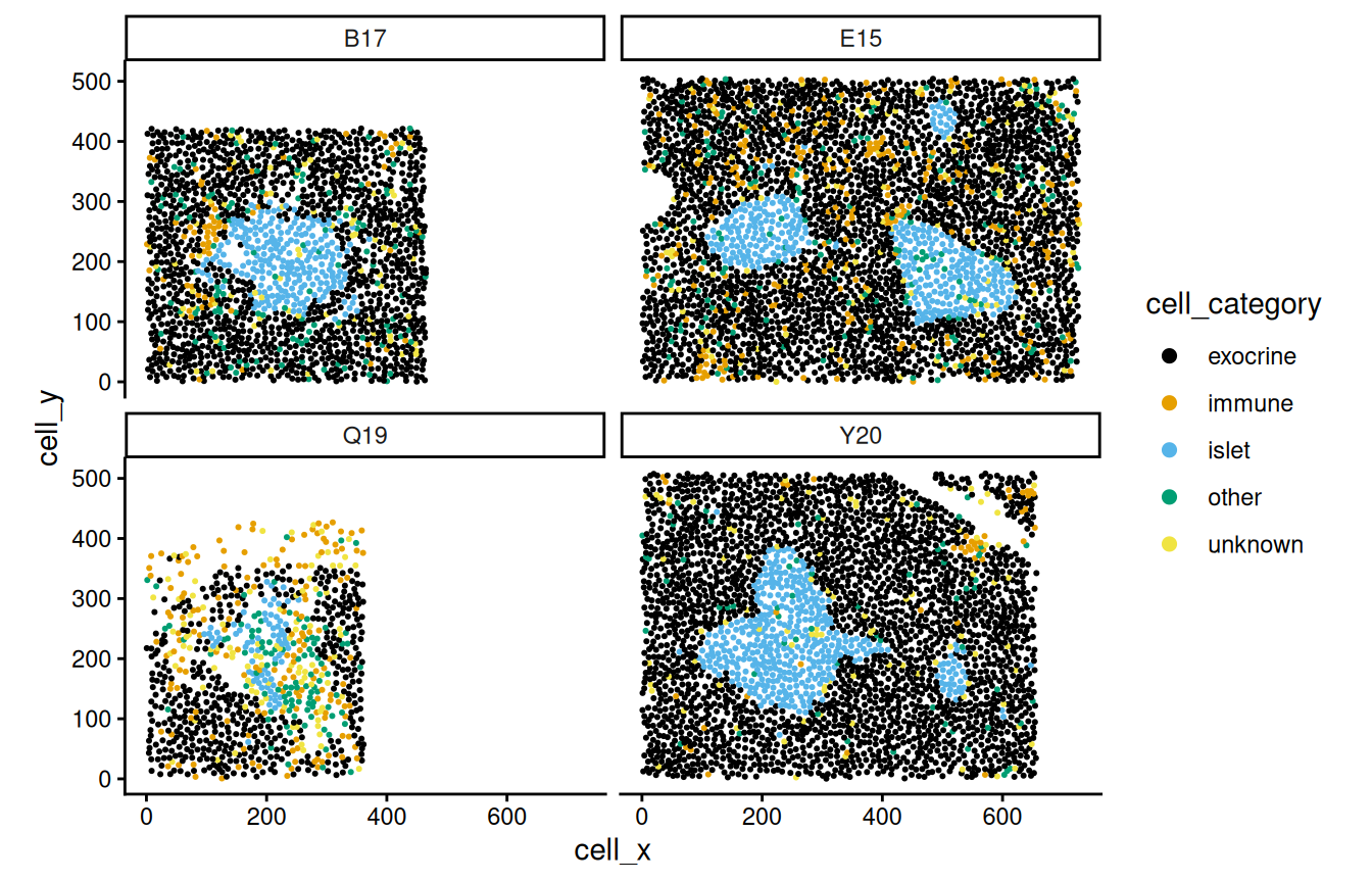
31.3 Islet reconstrution

Next we will reconstruct or segment the individual islet using a density-based approach implemented in sosta.

Code

n <- estimateReconstructionParametersSPE(
  spe, 
  marks = "cell_category", 
  imageCol = "image_name", 
  markSelect = "islet", 
  nImages = 10, # number of images for estimating parameters 
  nCores = 4
)

Code

thresSPE <- mean(n$thres)
bndwSPE <- mean(n$bndw)

Density based reconstruction

The sosta package uses a reconstruction method based on the point pattern density of the islet cells. This method needs two parameters – a bandwidth parameter that is used for the estimation of the intensity profile, and a threshold based on which the islets are reconstructed.

Code

shapeIntensityImage(
  spe, 
  marks = "cell_category", 
  imageCol = "image_name", 
  imageId = selPl[4], 
  markSelect = "islet"
)

Shown on the left is a density (pixel-level) image, and on the right a histogram of the intensity values. The method selects every pixel above a certain threshold for reconstruction. The smoothing bandwidth that generates the image is estimated using cross-validation (see function bw.diggle() of the spatstat.explore package from CRAN).

The threshold is estimated by taking the mean between the two modes of the (truncated) pixel intensity distribution. The function estimateReconstructionParametersSPE() repeats the estimation of these parameters for a selection of images in the dataset.

To make the reconstruction comparable between images we then use a fixed set of parameters for all images, in our case the mean of the individual parameters for a subset of the dataset.

Code

# run on all images
allIslets <- reconstructShapeDensitySPE(
  spe, 
  marks = "cell_category", 
  imageCol = "image_name", 
  markSelect = "islet", 
  bndw = bndwSPE, 
  thres = thresSPE, 
  nCores = 4
)

Now we can inspect the reconstruction in the sample images.

Code

df <- cbind(colData(spe[, spe$image_name %in% selPl]), 
            spatialCoords(spe[, spe$image_name %in% selPl]))

df |> 
  as.data.frame() |> 
  ggplot(aes(x = cell_x, y = cell_y, color = cell_category)) + 
  geom_point(size = 0.25) + 
  facet_wrap(~ image_name, ncol = 2) + 
  coord_equal() + 
  theme_classic() + 
  scale_color_manual(values=unname(pals::okabe(n = 5))) + 
  geom_sf(
    data = allIslets[allIslets$image_name %in% selPl, ], 
    inherit.aes = FALSE, 
    color = "firebrick", 
    fill = NA, 
    linewidth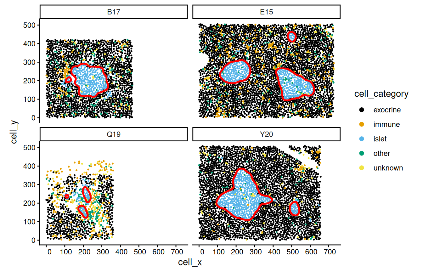 = 0.75
  )

##  Coordinate system already present. Adding new coordinate system, which will
##  replace the existing one.

The allIslets object is a simple feature collection which contains polygons (<GEOMETRY> column), a structure identifier (structID), and the image identifier (image_name). We will add some patient metadata to the object.

Code

colsKeep <- c(
  "patient_stage", 
  "tissue_slide", 
  "tissue_region", 
  "patient_id", 
  "patient_disease_duration", 
  "patient_age", 
  "patient_gender", 
  "sample_id"
)

# specify factor levels
lv <- c("Non-diabetic", "Onset", "Long-duration")

patientData <- colData(spe) |> 
  as_tibble() |> 
  group_by(image_name) |> 
  select(all_of(colsKeep)) |> 
  mutate(patient_stage = factor(patient_stage, levels = lv)) |> 
  unique()

##  Adding missing grouping variables: `image_name`

Code

allIslets <- allIslets |> 
  dplyr::left_join(patientData, by = "image_name")

31.4 Quantification of geometric features

Now we can proceed with quantification of geometric aspects of the islets and combine them with patient information.

Code

isletMetrics <- totalShapeMetrics(allIslets)
allIslets <- allIslets |> 
  cbind(t(isletMetrics))

PCA can give us an overview of the different features. Each dot represents one structure.

Code

autoplot(
  prcomp(t(isletMetrics), scale. = TRUE), 
  x = 1, 
  y = 2, 
  data = allIslets, 
  color = "patient_stage", 
  size = 2, 
  # shape = "type", 
  loadings = TRUE, 
  loadings.colour = "steelblue3", 
  loadings.label = TRUE, 
  loadings.label.size = 3, 
  loadings.label.repel = TRUE, 
  loadings.label.colour = "black"
) + 
  theme_bw() + 
  coord_fixed() + 
  scale_color_manual(values = unname(pals::tol(n = 3)))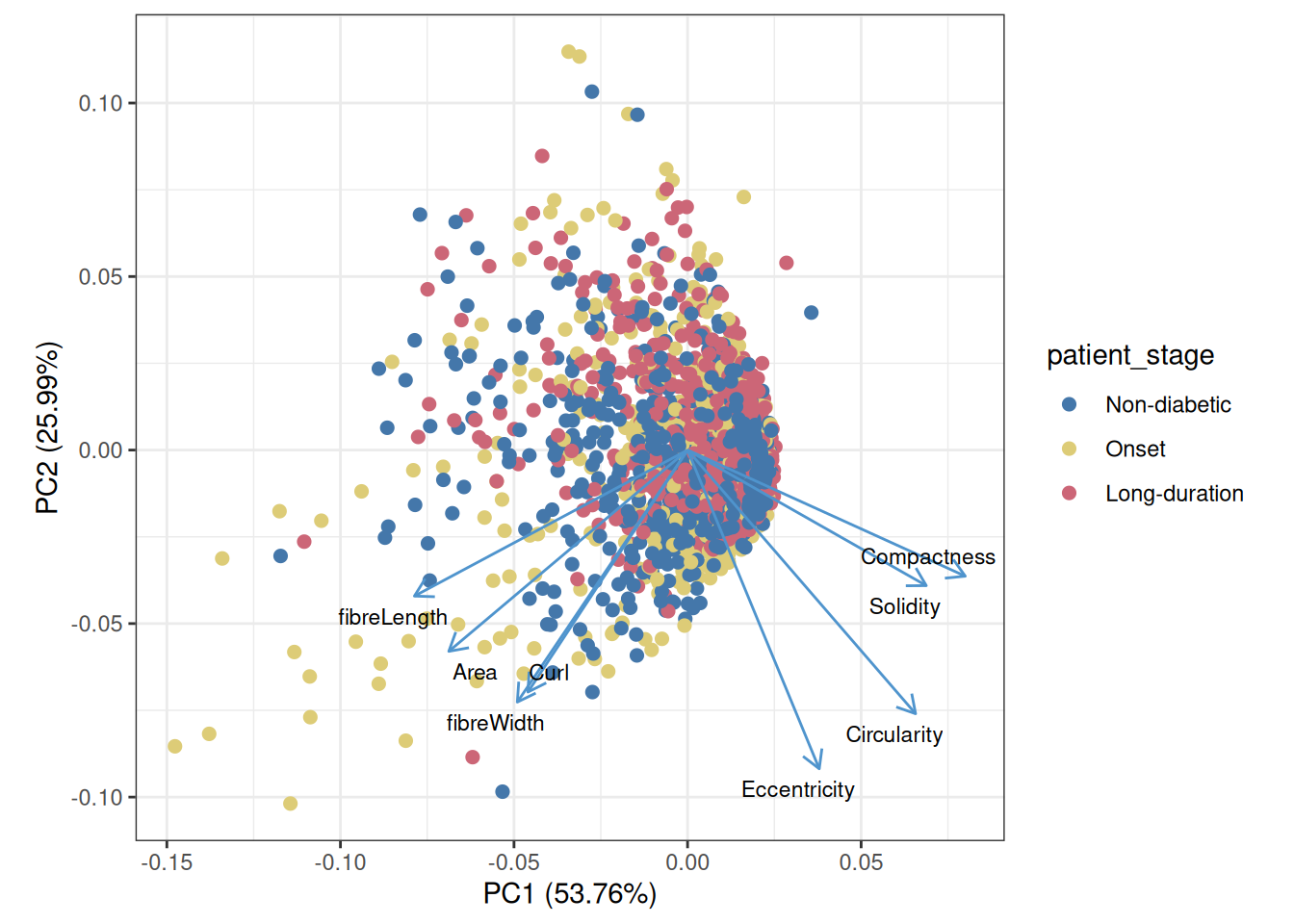

Code

allIslets |> 
  sf::st_drop_geometry() |> 
  select(patient_stage, rownames(isletMetrics)) |> 
  pivot_longer(-patient_stage) |> 
  filter(name %in% c("Area", "Compactness", "Curl")) |> 
  ggplot(aes(x = patient_stage, y = value, fill = patient_stage)) + 
  geom_violin() + 
  geom_boxplot(aes(fill = NULL), width = 0.3) + 
  facet_wrap( ~ name, scales = "free") + 
  scale_x_discrete(guide = guide_axis(n.dodge = 2)) + 
  guides(fill = "none") + 
  theme_bw() + 
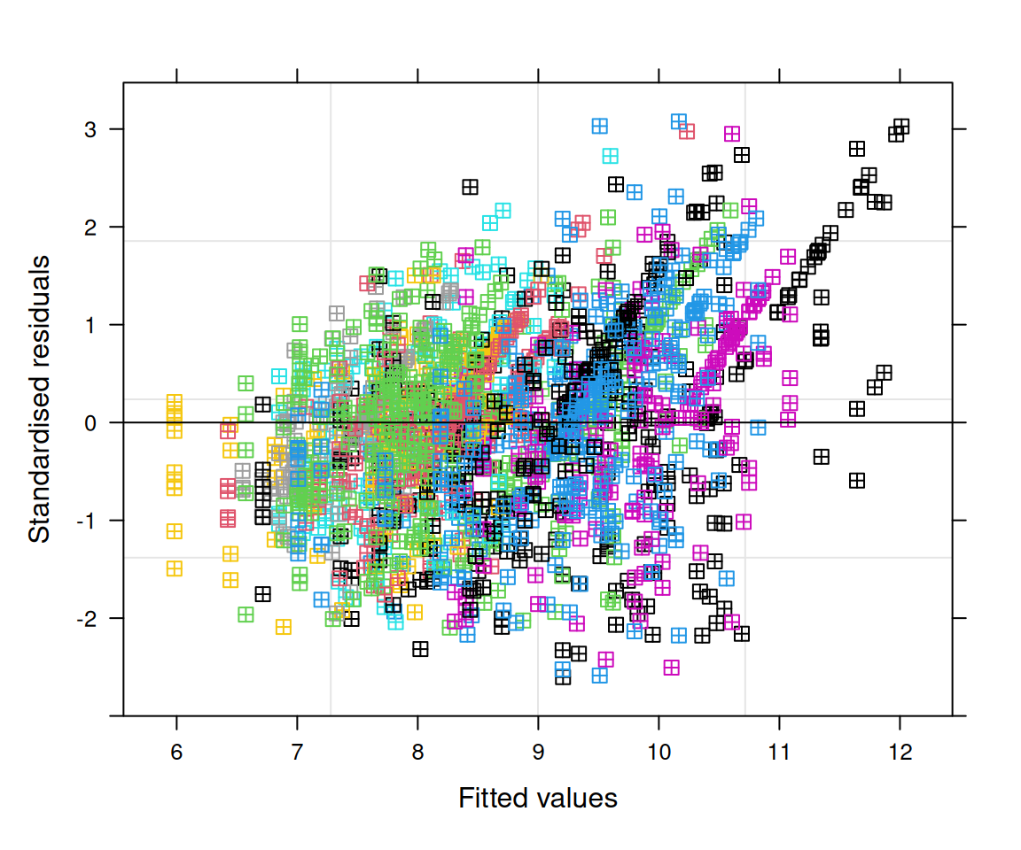
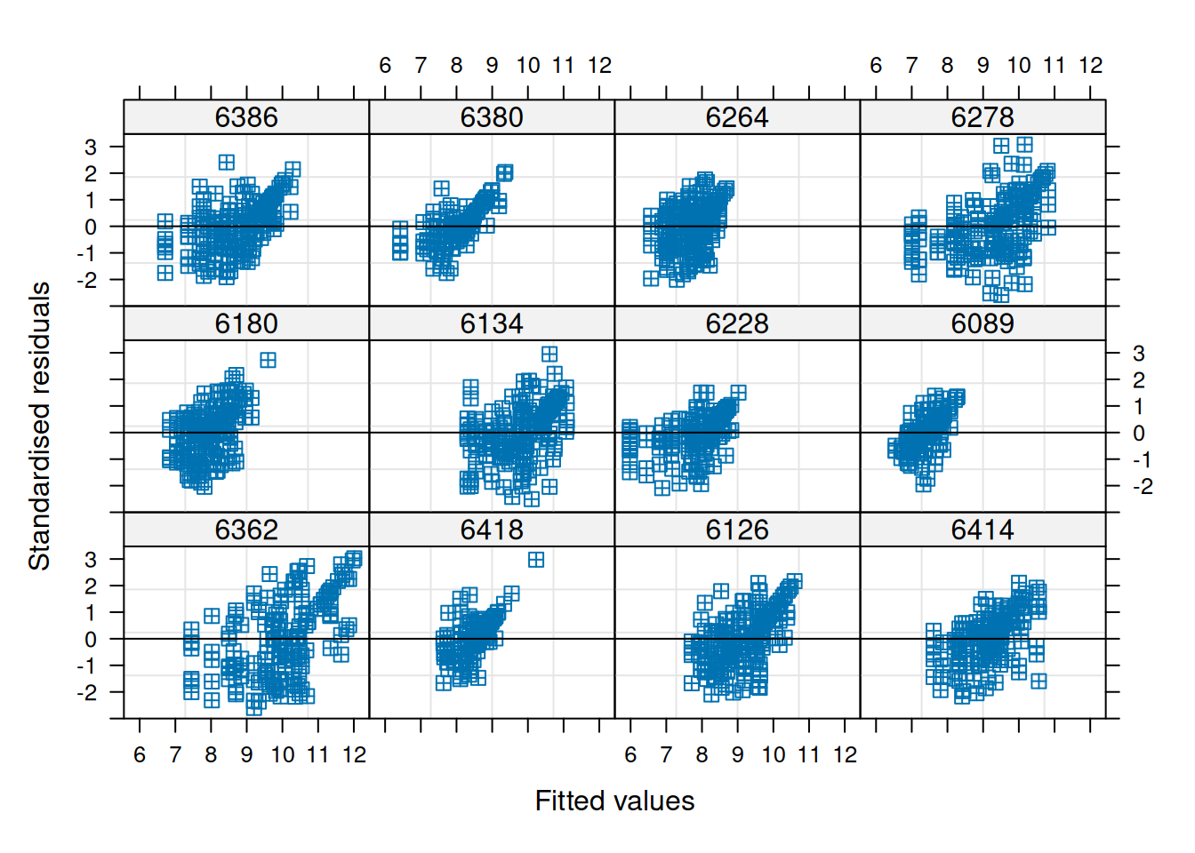
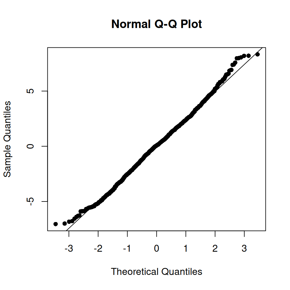
  scale_fill_manual(values = unname(pals::tol(n = 3)))

Let’s focus on the area of the islets and facet by patient to look at patient variability. As the distribution is very skewed we will use a 1/4-power transformation on the area of the islets. The transformation was chosen after inspection of the model diagnostics (see below).

Code

allIslets |> 
  sf::st_drop_geometry() |> 
  select(patient_stage, patient_id,  rownames(isletMetrics)) |> 
  pivot_longer(-c(patient_stage, patient_id)) |> 
  filter(name %in% c("Area")) |> 
  ggplot(aes(x = as.factor(patient_id), y = value^(1/4), fill = patient_stage)) + 
  geom_violin() + 
  geom_boxplot(aes(fill = NULL), width = 0.3) + 
  facet_wrap( ~ patient_stage, scales = "free") + 
  #scale_x_discrete(guide = guide_axis(n.dodge = 2)) + 
  guides(fill = "none") + 
  theme_bw() +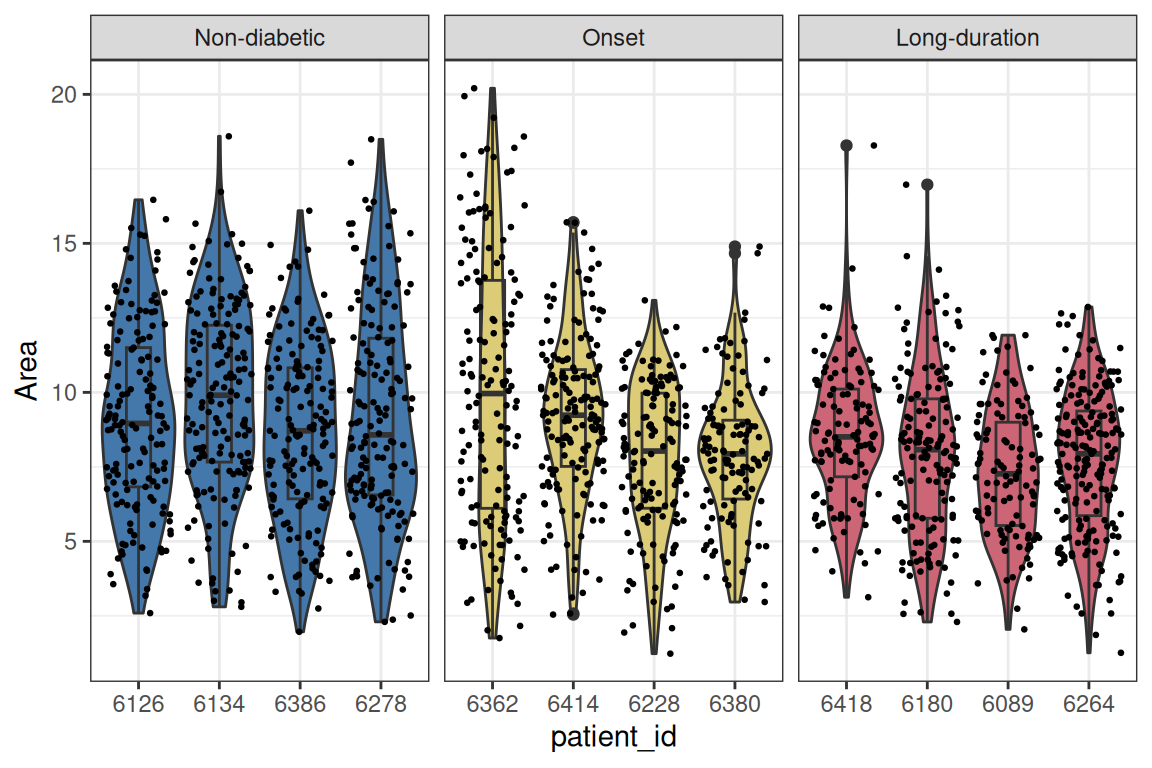 
  scale_fill_manual(values = unname(pals::tol(n = 3)))

31.5 Between-sample comparison using mixed effects models

The individual structure metrics are not independent measurements. Therefore, we have to account for correlation between measurements. This correlation stems from repeated measurements on the patient and slide level.

To account for this, we will use mixed linear models with random effects for the patient and the individual slides (image name). The lme4 package will be use for fitting linear mixed effects models (Bates et al. 2015) and lmerTest for p-value calculation (Kuznetsova, Brockhoff, and Christensen 2017).

Code

mod <- lmer((Area)^(1/4) ~ patient_stage + (1 | patient_id) + (1 | image_name), 
            data = allIslets)

Model diagnostics

31.6 Residuals vs. fitted

Code

plot(
  mod, 
  resid(., scaled = TRUE) ~ fitted(.), 
  col = allIslets$patient_id, 
  pch = 12, 
  abline = 0, 
  xlab = "Fitted values", 
  ylab = "Standardised residuals"
)

31.7 Residuals vs. fitted per sample

Code

plot(
  mod, 
  resid(., scaled = TRUE) ~ fitted(.) | patient_id, 
  abline = 0, 
  pch = 12, 
  xlab = "Fitted values", 
  ylab = "Standardised residuals"
)

31.8 QQ plot

Code

qqnorm(resid(mod), pch = 16)
qqline(resid(mod))

Code

summary(mod)

##  Linear mixed model fit by REML. t-tests use Satterthwaite's method [
##  lmerModLmerTest]
##  Formula: (Area)^(1/4) ~ patient_stage + (1 | patient_id) + (1 | image_name)
##     Data: allIslets
##  
##  REML criterion at convergence: 9028
##  
##  Scaled residuals: 
##      Min      1Q  Median      3Q     Max 
##  -2.6027 -0.6199  0.0265  0.6129  3.0764 
##  
##  Random effects:
##   Groups     Name        Variance Std.Dev.
##   image_name (Intercept) 1.4628   1.2095  
##   patient_id (Intercept) 0.5426   0.7366  
##   Residual               7.3230   2.7061  
##  Number of obs: 1806, groups:  image_name, 844; patient_id, 12
##  
##  Fixed effects:
##                             Estimate Std. Error      df t value Pr(>|t|)    
##  (Intercept)                  9.5935     0.3924  8.8393  24.447 2.01e-09 ***
##  patient_stageOnset          -0.5624     0.5557  8.8860  -1.012    0.338    
##  patient_stageLong-duration  -1.5404     0.5563  8.9198  -2.769    0.022 *  
##  ---
##  Signif. codes:  0 '***' 0.001 '**' 0.01 '*' 0.05 '.' 0.1 ' ' 1
##  
##  Correlation of Fixed Effects:
##              (Intr) ptnt_O
##  ptnt_stgOns -0.706       
##  ptnt_stgLn- -0.705  0.498

From the fixed effects section in summary(mod) we note that there is a statistically significant difference in the transformed islet area of long-duration patients with respect to non-diabetic patients, while the effect for onset patients is not significant at the 5% level. This results accounts for correlation at the patient and image level as modeled by random intercepts. The transformation (1/4-power) was chosen after inspection of the residual behavior in the model diagnostics for this dataset and feature of interest specifically.

31.9 Appendix

31.9.1 Other packages

Additional packages to calculate anatomical structure-derived features include:

The Bioconductor packages SPIAT and imcRtools offer other functions to quantify features on the anatomical structure level. These could also be input for mixed effect modeling as illustrated above.
The packages vegan and poem are useful when calculating diversity metrics within structures and / or border regions. To identify border regions and how to overlap anatomical regions with sample coordinates please have a look at the sosta vignette.

31.9.2 Notes

This chapter is based on the sosta vignette “2. Reconstruction and analysis of pancreatic islets from IMC data”.

References

Bates, Douglas, Martin Mächler, Ben Bolker, and Steve Walker. 2015. “Fitting Linear Mixed-Effects Models Using Lme4.” Journal of Statistical Software 67 (1). https://doi.org/10.18637/jss.v067.i01.

Damond, Nicolas, Stefanie Engler, Vito R. T. Zanotelli, Denis Schapiro, Clive H. Wasserfall, Irina Kusmartseva, Harry S. Nick, et al. 2019. “A Map of Human Type 1 Diabetes Progression by Imaging Mass Cytometry.” Cell Metabolism 29 (3): 755–768.e5. https://doi.org/10.1016/j.cmet.2018.11.014.

Kuznetsova, Alexandra, Per B. Brockhoff, and Rune H. B. Christensen. 2017. “lmerTest Package: Tests in Linear Mixed Effects Models.” Journal of Statistical Software 82 (December): 1–26. https://doi.org/10.18637/jss.v082.i13.