21  Cell-cell communication

21.1 Preamble

21.1.1 Introduction

Having identified spatial patterns in cellular organization and gene expression, it is further of interest to characterize how cells coordinate activity through i) their (physical) community context, or cell-cell interactions (CCI); and, ii) protein-mediated signaling, or cell-cell communication (CCC).

Mechanisms underlying inter-cellular interaction and communication have been classified as autocrine, juxtacrine, paracrine, and endocrine to refer to intra-cellular, contact-dependent, close- and long-range signaling events, respectively (Armingol et al. 2020). Paracrine events, for instance, depend on diffusion of signaling molecules between proximal cells; endocrine events are mediated by molecules (typically hormones) that travel between distal cells through extracellular fluids.

In scRNA-seq data, CCI/C is commonly studied through ligand-receptor (LR) pairs, but corresponding tools are restricted to gene expression only; e.g., CellphoneDB (Efremova et al. 2020). However, incorporating spatial information should enrich this type of analysis because distances between cells play a key role in inter-cellular signaling.

Methods developed for CCI/C analysis of spatial (transcript)omics data consider cellular distances to adjust interactions predicted from expression, and typically aim at quantifying spatial co-expression of LRs (that is, between proximal cells). Such analyses need not be limited to LRs, however.

In principle, any CCC tool may be turned into a spatial one by:

  1. pre-filtering: select a spatial neighborhood,
    and apply CCC inference to selected observations.

  2. post-filtering: apply CCC inference,
    and filter results based on spatial proximity.

The reason we might choose to take one of these approaches is because CCC modeling frameworks designed for single cell data are typically less complex. Consequently, they tend to be more interpretable, easier and faster to run.

21.1.2 Dependencies

Code
library(dplyr)
library(tidyr)
library(scater)
library(scuttle)
library(CCPlotR)
library(ggplot2)
library(ggspavis)
library(patchwork)
library(reticulate)
library(BiocParallel)
library(zellkonverter)
library(SpatialExperiment)
# load data from previous chapter
# (past quality control & clustered)
spe <- readRDS("img-spe_cl.rds")
# specify whether/how to 
# perform parallelization
bp <- MulticoreParam(4)

21.2 COMMOT

Here we run COMMOT (Cang et al. 2023), an optimal transport-based approach that models competition between sender and receiver signals, can account for multimeric interactions, considers cell-cell distances, and is linked to databases of signalling interactions and pathways.

Since COMMOT is available as a Python package, we can access it from R using reticulate with a Conda environment (see Chapter 7).

21.2.1 Python setup

We first set up a Python environment. Here, we do this by re-using the Conda environment created in Chapter 7, in order to speed up the book build time. Alternatively, a new environment could also be set up instead (see Chapter 7).

We also install the commot package and additional dependencies from PyPI.

Alternatively, one could set up a conda environment (or similar) outside of R, following the authors’ installation instructions for COMMOT, and activate it with reticulate::use_condaenv().

Code
# re-use environment from Python interoperability chapter
# using reticulate functions
env <- "env-ccc"
conda_clone(env, clone = "py-interop")
##  [1] "/root/.local/share/r-miniconda/envs/env-ccc/bin/python"
Code
use_condaenv(env, required = TRUE)

# install additional Python packages from PyPI
conda_install(
  envname = env, 
  packages = c("commot==0.0.3", "anndata==0.12.2", "pandas==2.3.2", "numpy==1.26.4"), 
  pip = TRUE
)
##  [1] "'commot==0.0.3'"   "'anndata==0.12.2'" "'pandas==2.3.2'"  
##  [4] "'numpy==1.26.4'"

21.2.2 LR retrieval

First, we retrieve ligand-receptor interactions (and a lot more!) from CellChatDB (Jin et al. 2021) using COMMOT’s ligand_receptor_database() function.

Code
# retrieve LR interaction from CellChatDB
ct <- import("commot")
db <- ct$pp$ligand_receptor_database(
    species="human", 
    database="CellChat", 
    signaling_type=NULL)
names(db) <- c("ligand", "receptor", "pathway", "type")
head(db)
##    ligand      receptor pathway               type
##  0  TGFB1 TGFBR1_TGFBR2    TGFb Secreted Signaling
##  1  TGFB2 TGFBR1_TGFBR2    TGFb Secreted Signaling
##  2  TGFB3 TGFBR1_TGFBR2    TGFb Secreted Signaling
##  3  TGFB1 ACVR1B_TGFBR2    TGFb Secreted Signaling
##  4  TGFB1 ACVR1C_TGFBR2    TGFb Secreted Signaling
##  5  TGFB2 ACVR1B_TGFBR2    TGFb Secreted Signaling

While we obtain 1939 interactions from above, the vast majority of genes involved are missing from our panel. Filtering for those that are fully covered, we are left with very few:

Code
# interaction types &
# number of interactions
table(db$type)
##  
##   Cell-Cell Contact       ECM-Receptor Secreted Signaling 
##                 319                421               1199
Code
# number of unique features
lr <- c(db$ligand, db$receptor)
ss <- strsplit(lr, "-")
gs <- sapply(ss, .subset, 1)
length(unique(unlist(gs)))
##  [1] 983
Code
# filer for those fully covered by the panel
keep <- apply(db, 1, \(.) {
    rs <- strsplit(.["receptor"], "_")
    lr <- c(.["ligand"], unlist(rs))
    all(lr %in% rownames(spe))
})
(db <- db[keep, ])
##         ligand receptor pathway               type
##  711    CXCL12    CXCR4    CXCL Secreted Signaling
##  882       PTN     SDC4     PTN Secreted Signaling
##  905      EDN1    EDNRB     EDN Secreted Signaling
##  1640    PTPRC     MRC1    CD45  Cell-Cell Contact
##  1644     CD80    CD274    CD80  Cell-Cell Contact
##  1646     CD80    CTLA4    CD80  Cell-Cell Contact
##  1648     CD86    CTLA4    CD86  Cell-Cell Contact
##  1657     CDH1     CDH1     CDH  Cell-Cell Contact
##  1671     CD69    KLRB1    CLEC  Cell-Cell Contact
##  1834    NCAM1    NCAM1    NCAM  Cell-Cell Contact
##  1887    CD274    PDCD1   PD-L1  Cell-Cell Contact
##  1888 PDCD1LG2    PDCD1    PDL2  Cell-Cell Contact
##  1889   PECAM1   PECAM1  PECAM1  Cell-Cell Contact

21.2.3 CCC inference

To reduce runtime, we will restrict analysis to a 2mm\(2\) tissue section:

Code
# subset data to features being considered
ss <- strsplit(db$receptor, "_")
rs <- sapply(ss, .subset, 1)
sub <- spe[unique(c(db$ligand, rs)), ]

# assign spatial coordinates to 'spatial' 
# reduced dimension slot (required by 'COMMOT')
xy <- spatialCoords(sub)
reducedDim(sub, "spatial") <- xy

# get indices of cells that fall
# into a (2mm) x (2mm) window
cs <-
    xy[, 1] >= 1500 & xy[, 1] <= 3500 &
    xy[, 2] >= 2000 & xy[, 2] <= 4000

# print number of genes x cells left
dim(sub <- sub[, cs]) 
##  [1]    19 15003

We now perform run CCC inference, using zellkonverter’s SCE2AnnData function to convert our spe in R to an AnnData object in Python. Note that in real settings (e.g., lots of interactions across lots of cells), this can be parallelized, e.g., across fields of view (FOVs) or tissue sections.

For documentation on parameter meaning and choices, see the tutorial.
Code
# convert 'SpatialExperiment' (R) to 
# 'AnnData' (Python) using 'zellkonverter'
ad <- SCE2AnnData(sub, X_name="logcounts")
# run CCC inference using 'COMMOT'
ct <- import("commot")
ct$tl$spatial_communication(ad,
    database_name="CellChatDB",
    dis_thr=10,  
    df_ligrec=db,
    heteromeric=TRUE,
    pathway_sum=TRUE,
    heteromeric_rule="min",
    heteromeric_delimiter="_")
# extract 'data.frame's containing
# sender & receiver CCC estimates
ccc <- list(
    s=ad$obsm["commot-CellChatDB-sum-sender"],
    r=ad$obsm["commot-CellChatDB-sum-receiver"])
# add CCC inference results as cell metadata
for (df in ccc) colData(sub)[names(df)] <- df

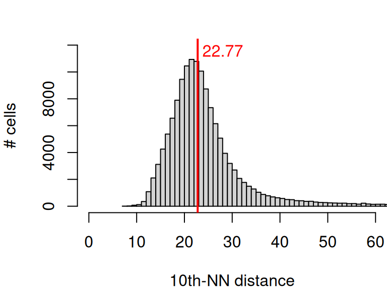
An important consideration is the distance threshold to impose on CCC inference (argument dis_thr in the code chunk below). Ideally, this decision is based on a biological expectation on cell size and signalling range. Estimates on the distance over which immune cell signaling can occur, for example, measured interactions on length scales of 80-120\(\mu\)m (Oyler-Yaniv et al. 2017).

Alternatively, we can arrive at a data-driven estimate by inspecting the distribution of \(k\)th-NN distances for a sensible \(k\) that, in this context, determines the number of cells to consider as potential communication partners:

Code
xy <- spatialCoords(spe)
ns <- RANN::nn2(xy, xy, 11)
ds <- ns$nn.dists[, 11]
par(mar=c(4,4,2,0))
hist(ds, n=200,
    xlim=c(0, 60), ylim=c(0, 12e3),
    xlab="10th-NN distance", 
    ylab="# cells", main="")
abline(v=d <- median(ds), lw=2, col="red")
text(d+1, 12e3, adj=c(0,1), round(d, 2), col="red")

21.3 Visualization

21.3.1 In space

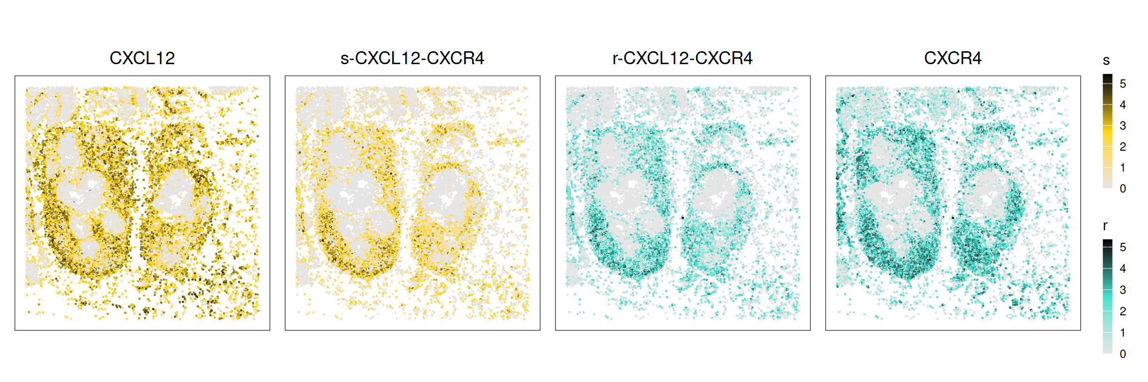
Visualizing the above data across the tissue, we will typically observe that expression and signalling values give similar spatial patterns, but the latter will be restricted to where ligand and receptor-expressing cells co-localize.

For simplicity, we pick a single interaction (CXCL12-CXCR4 signalling); here, s and r correspond to sender and receiver signal, respectively:

Code
# specify colors for sender/receiver signals
pal <- list(
    s=c("grey90", "gold", "black"), 
    r=c("grey90", "turquoise", "black"))

# get variables names of the form: x, s-x-y, r-x-y, y
.f <- \(i, j) c(i, paste(c("s","r"), i,j, sep="-"), j)
xs <- .f("CXCL12", "CXCR4")

# visualize expression & signaling side-by-side
lapply(seq_along(xs), \(.) {
    typ <- ifelse(. < 3, "s", "r")
    plotCoords(sub, point_size=0.5,
        annotate=xs[.], assay_name="logcounts") + 
        scale_color_gradientn(typ, colors=pal[[typ]])
}) |>
    wrap_plots(nrow=1, guides="collect")  &
    theme(legend.key.width=unit(0.5, "lines"))

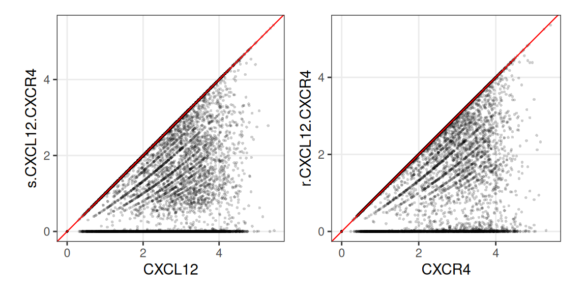
Let’s compare gene expression values with cell-cell signalling estimates:

Code
es <- t(as.matrix(logcounts(sub)))
df <- data.frame(colData(sub), es)
ggplot(df, aes(CXCL12, s.CXCL12.CXCR4)) + 
ggplot(df, aes(CXCR4, r.CXCL12.CXCR4)) + 
    plot_layout(nrow=1) &
    geom_point(shape=16, stroke=0, size=1, alpha=0.2) &
    geom_abline(intercept=0, slope=1, linewidth=0.4, col="red") &
    coord_equal() & theme_bw() & theme(panel.grid.minor=element_blank())

We can observe that x- and y-values are similar for only a subset of cells. A portion of cells expresses CXCL12/CXCR4, but takes on 0 signalling values. In between, signalling estimates fall below the corresponding expression values.

This makes sense, knowing that COMMOT considers physical cell-cell distances. I.e., some cells express CXCL12/CXCR4, but are too distant from cells expressing CXCR4/CXCL12, and are thus deemed to not be involved in signalling. Meanwhile, there is a penalty on signalling in proportion to the distance between sender and receiver cells, as well as competition between proximal cells, yielding non-zero but lower-than-expression values.

21.3.2 In general

From a biological perspective, we might be less interested signaling at the single cell-level. Instead, we could explore (for example but not limited to):

  • Which subpopulations are signaling to one another?
  • How does signaling at the subpopulation-level compare across niches (i.e., different spatial contexts) or pathologies (e.g., healthy/tumor)?
  • How does signaling compare across different sections (e.g., patients)?

In essence, CCC results correspond to another assay, and we can compare them the same way we would compare gene expression across subpopulations, niches, regions of interest, sections, etc.

In order to more easily investigate this, we can reformat estimates for sender and receiver signals from CCC inference into a SingleCellExperiment object where rows = interactions and columns = cells.

Code
# construct SCE from CCC results;
# assays = s(ender) & r(eceiver)
as <- lapply(ccc, \(.) {
    names(.) <- gsub("^(s|r)-", "", names(.))
    as(t(as.matrix(.)), "dgCMatrix")
})
(sce <- SingleCellExperiment(as, colData=colData(sub)))
##  class: SingleCellExperiment 
##  dim: 26 15003 
##  metadata(0):
##  assays(2): s r
##  rownames(26): CD69-KLRB1 CD80-CTLA4 ... PECAM1 PTN
##  rowData names(0):
##  colnames(15003): 4303 4305 ... 107719 107722
##  colData names(69): cell_id transcript_counts ... r-PECAM1 r-PTN
##  reducedDimNames(0):
##  mainExpName: NULL
##  altExpNames(0):

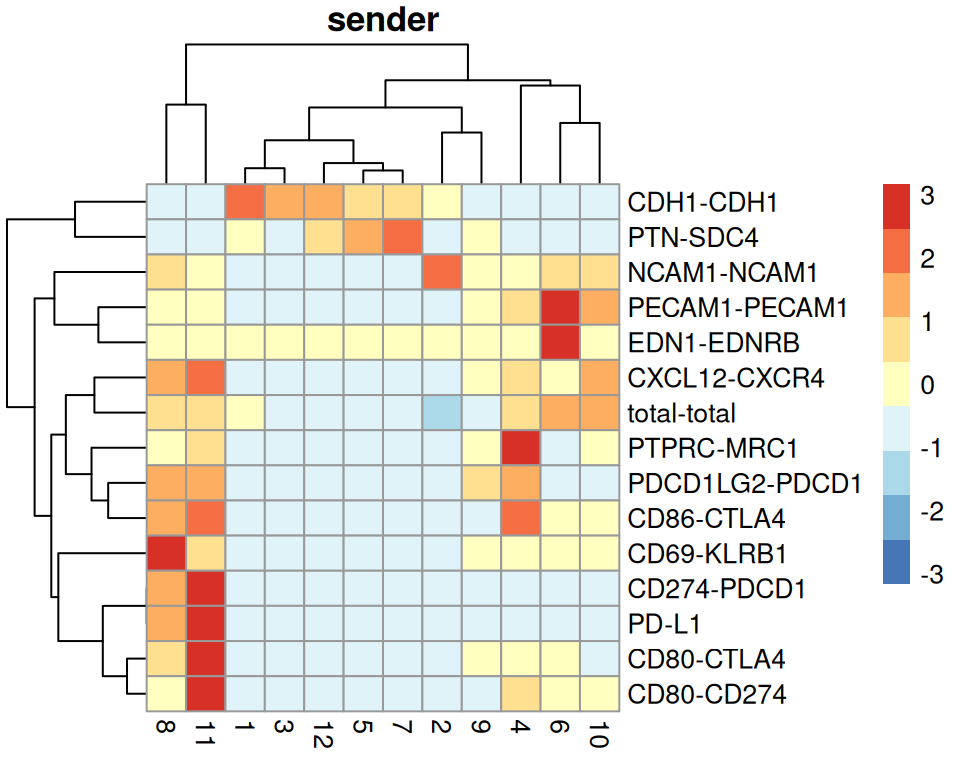
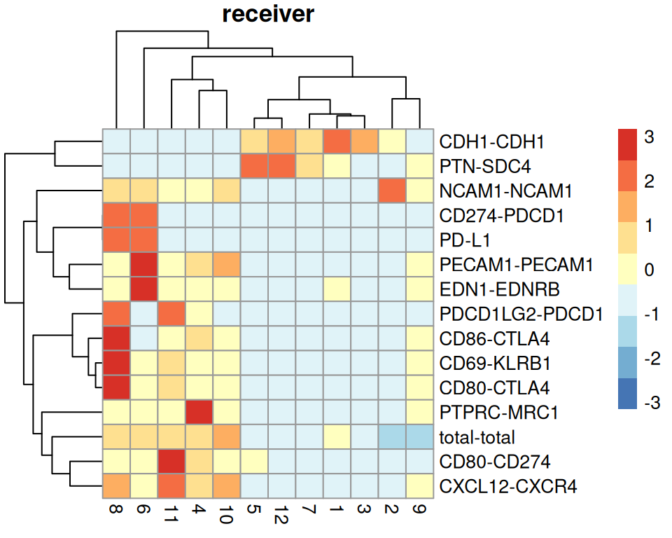
Next, we summarize CCC results for each subpopulation (separately for sender and receiver estimates) and visualize subpopulation-level results in a heatmap, using SCE-friendly functions for aggregation and visualization available through packages like scuttle and scater.

Code
# aggregate estimates by cluster
# (separately for sender/receiver)
mu <- aggregateAcrossCells(sce, 
    ids=sce$Leiden, 
    statistics="mean",
    use.assay.type=assayNames(sce))

# visualize scales values across clusters
for (. in assayNames(mu)) {
    plotHeatmap(mu, exprs_values=.,
        features=grep("-", rownames(sce)),
        main=switch(., s="sender", r="receiver"),
        show_colnames=TRUE, center=TRUE, scale=TRUE)
}

The CCPlotR (Ennis, Ó Broin, and Szegezdi 2023) package provides a visualization suit for CCC analysis results, including graphs and circos plots. These rely on a generic format, where each row contains the source and target cluster, sender and receiver feature, as well as an interaction score. It is not straightforward how to best arrive at the latter; naively, we can simply average across sender and receiver estimates, either at the single cell- or cluster-level, to obtain such a score:

Code
# average across cluster-level sender/receiver 
# averages to obtain i(nteraction) scores
ks <- expand.grid(ks <- colnames(mu), ks)
cs <- split(colnames(sce), sce$Leiden)
lr <- grepl("-", rownames(sce))
lr <- lr & !grepl("total", rownames(sce))
ss <- strsplit(rownames(sce), "-")
l <- sapply(ss, .subset, 1)
r <- sapply(ss, .subset, 2)
df <- mapply(
    i=ks[, 1], j=ks[, 2],
    SIMPLIFY=FALSE, \(i, j) {
        source <- sce[lr, cs[[i]]]
        target <- sce[lr, cs[[j]]]
        sr <- cbind(
            rowMeans(assay(source, "s")),
            rowMeans(assay(target, "r")))
        data.frame(
            source=paste(i), target=paste(j),
            ligand=l[lr], receptor=r[lr],
            score=rowMeans(sr))
    }) |> do.call(what=rbind)
rownames(df) <- NULL
head(df)
##    source target ligand receptor      score
##  1      1      1   CD69    KLRB1 0.00000000
##  2      1      1   CD80    CTLA4 0.00000000
##  3      1      1   CD80    CD274 0.00000000
##  4      1      1 PECAM1   PECAM1 0.01452581
##  5      1      1  CD274    PDCD1 0.00000000
##  6      1      1   CDH1     CDH1 2.10121365

We are now set to generate a range of visualizations using CCPlotR, e.g., a circos plot where the width of the links represents the total number of interactions between clusters. However, because this is only a toy example (few genes and cells), we will refrain from any biological interpretation.

Code
cc_circos(df, n_top_ints=100)

On a final note, inference is arguably much more complex (and results less straightforward to interpret) when a higher-plex panel is being considered; i.e., when overlapping and multimeric interactions are involved, which did not apply in the example provided here. Nevertheless, we hope that readers can appreciate the conceptual difference between expression data and CCC results, and will be able to implement similar reticulate approaches to incorporate methods living in Python into their analysis pipelines.

21.4 Appendix

  • Liu, Sun, and Wang (2022) compare methods developed for CCC analysis of spatially resolved data with non-spatial approaches.

  • mistyR (Tanevski et al. 2022) distinguishes between an ‘intrinsic’ view to capture how markers within a location influence one another; a ‘juxtaview’ to model local cellular niche (by relating expression between neighboring cells); and, a ‘paraview’ to capture tissue structure effects (by relating expression within a given radius).

  • Giotto (Chen2023-Giotto-Suite?) detects increased co-expression of LR pairs in neighboring cells of different types via comparison to randomly shuffled cell locations (permutation test).

  • CellChat (Jin, Plikus, and Nie 2025) quantifies CCC signalling probability between two groups of cells using a simplified mass action-based model, which incorporates core LR interaction with potential multimeric structure and modulation by cofactors.

  • SpatialDM (Li et al. 2023) uses a bivariate extension of Moran’s \(I\) – a measure of spatial autocorrelation (cf., Chapter 29) – to test LR pairs in close-range distance against independence.

  • SpaOTsc (Cang and Nie 2020) relies on optimal transport to segregate signal in a spatial region into LRs and their downstream genes, yielding information on regulatory flows between cells.

References

Armingol, Erick, Adam Officer, Olivier Harismendy, and Nathan E Lewis. 2020. “Deciphering Cell–Cell Interactions and Communication from Gene Expression.” Nature Reviews Genetics 22 (2): 71–88. https://doi.org/10.1038/s41576-020-00292-x.
Cang, Zixuan, and Qing Nie. 2020. “Inferring Spatial and Signaling Relationships Between Cells from Single Cell Transcriptomic Data.” Nature Communications 11 (2084). https://doi.org/10.1038/s41467-020-15968-5.
Cang, Zixuan, Yanxiang Zhao, Axel A. Almet, Adam Stabell, Raul Ramos, Maksim V. Plikus, Scott X. Atwood, and Qing Nie. 2023. “Screening Cell–Cell Communication in Spatial Transcriptomics via Collective Optimal Transport.” Nature Methods 20: 218–28. https://doi.org/10.1038/s41592-022-01728-4.
Efremova, Mirjana, Miquel Vento-Tormo, Sarah A Teichmann, and Roser Vento-Tormo. 2020. CellPhoneDB: Inferring Cell-Cell Communication from Combined Expression of Multi-Subunit Ligand-Receptor Complexes.” Nature Protocols 15 (4): 1484–1506. https://doi.org/10.1038/s41596-020-0292-x.
Ennis, Sarah, Pilib Ó Broin, and Eva Szegezdi. 2023. CCPlotR: An R Package for the Visualization of Cell-Cell Interactions.” Bioinformatics Advances 3 (1): vbad130. https://doi.org/10.1093/bioadv/vbad130.
Jin, Suoqin, Christian F Guerrero-Juarez, Lihua Zhang, Ivan Chang, Raul Ramos, Chen-Hsiang Kuan, Peggy Myung, Maksim V Plikus, and Qing Nie. 2021. “Inference and Analysis of Cell-Cell Communication Using CellChat.” Nature Communications 12 (1): 1088. https://doi.org/10.1038/s41467-021-21246-9.
Jin, Suoqin, Maksim V Plikus, and Qing Nie. 2025. CellChat for Systematic Analysis of Cell-Cell Communication from Single-Cell Transcriptomics.” Nature Protocols 20 (1): 180–219. https://doi.org/10.1038/s41596-024-01045-4.
Li, Zhuoxuan, Tianjie Wang, Pengtao Liu, and Yuanhua Huang. 2023. SpatialDM: Rapid Identification of Spatially Co-Expressed Ligand-Receptor Reveals Cell-Cell Communication Patterns.” bioRxiv, 2022.08.19.504616. https://doi.org/10.1101/2022.08.19.504616.
Liu, Zhaoyang, Dongqing Sun, and Chenfei Wang. 2022. “Evaluation of Cell-Cell Interaction Methods by Integrating Single-Cell RNA Sequencing Data with Spatial Information.” Genome Biology 23 (1): 218. https://doi.org/10.1186/s13059-022-02783-y.
Oyler-Yaniv, Alon, Jennifer Oyler-Yaniv, Benjamin M Whitlock, Zhiduo Liu, Ronald N Germain, Morgan Huse, Grégoire Altan-Bonnet, and Oleg Krichevsky. 2017. “A Tunable Diffusion-Consumption Mechanism of Cytokine Propagation Enables Plasticity in Cell-to-Cell Communication in the Immune System.” Immunity 46 (4): 609–20. https://doi.org/10.1016/j.immuni.2017.03.011.
Tanevski, Jovan, Ricardo Omar Ramirez Flores, Attila Gabor, Denis Schapiro, and Julio Saez-Rodriguez. 2022. “Explainable Multiview Framework for Dissecting Spatial Relationships from Highly Multiplexed Data.” Genome Biology 23 (1): 97. https://doi.org/10.1186/s13059-022-02663-5.
Back to top