27  Normalization

27.1 Preamble

27.1.1 Introduction

Normalization is a critical step in the analysis of transcriptomics and other high-throughput biological data, aiming to remove technical variability while preserving true biological signals.

In single-cell RNA sequencing, normalization aims at removing differences in sequencing coverage between libraries (cells). Such differences in library size are typically accounted for by scaling the counts in each cell by a size factor, which is often computed as the total number of counts for that cell (or a robust variant thereof); see OSCA.

Single-cell normalization methods have been widely used for the analysis of spatial transcriptomics (ST) data, given the similarity between the two technologies, which both yield count data. While this is justifiable for sequencing-based ST technologies, it is less clear that this is appropriate for imaging-based ones.

In fact, in imaging-based ST, the total number of counts is driven by the number of probes that successfully hybridize to their target transcripts within each cell and not by the sequencing coverage. It is hence less clear that this leads to the same compositional biases as in sequencing platforms. Moreover, these technologies often employ targeted gene panels rather than whole-transcriptome profiling, which may lead to confounding between total counts and biology, as shown by Atta et al. (2024) and Bhuva et al. (2024).

Here, we will review both scaling normalization methods and spatially-aware normalization methods that have been specifically developed for ST data.

27.1.2 Dependencies

library(ggplot2)
library(OSTA.data)
library(patchwork)
library(scrapper)
library(SpatialExperiment)
# load data from preceding 
# chapter (post quality control)
(spe <- readRDS("img-spe_qc.rds"))

##  class: SpatialExperiment 
##  dim: 313 140268 
##  metadata(1): qc
##  assays(1): counts
##  rownames(313): ABCC11 ACTA2 ... ZEB2 ZNF562
##  rowData names(3): ID Symbol Type
##  colnames(140268): 2 3 ... 167779 167780
##  colData names(12): cell_id transcript_counts ... detected keep
##  reducedDimNames(0):
##  mainExpName: NULL
##  altExpNames(0):
##  spatialCoords names(2) : x_centroid y_centroid
##  imgData names(1): sample_id

# get annotations from 'BiocFileCache'
# (data has been retrieved already)
id <- "Xenium_HumanBreast1_Janesick"
pa <- OSTA.data_load(id, mol=FALSE)
dir.create(td <- tempfile())
unzip(pa, "annotation.csv", exdir=td)
df <- read.csv(list.files(td, full.names=TRUE))
# add annotations as cell metadata
cs <- match(spe$cell_id, df$Barcode)
spe$Label <- df$Annotation[cs]

27.2 Scaling normalization

As a baseline, we will apply log-library size normalization, as implemented in the scrapper package. Note that the normalizeRnaCounts.se function adds a new assay named logcounts to the spe object, which contains the normalized expression values on the log scale.

spe <- normalizeRnaCounts.se(spe)
spe$sf_lib <- sizeFactors(spe)
assayNames(spe)

##  [1] "counts"    "logcounts"

NoteLog-library size normalization

Log-library size normalization is the simplest normalization strategy and the default option in several single-cell RNA-seq workflows. It normalizes the data by dividing each count by the column sums and rescaling them so that the original scale of the counts is preserved. Finally, the resulting normalized data are log-transformed after adding a pseudo-count, typically one, to avoid issues with the log of zero.

Specifically, denoting with \(y_{ij}\) the count of gene \(j\) in cell \(i\), with \(y_{i.}\) the sum of all gene counts for cell \(i\) (library size), and with \(y_{..}\) the sum of all counts across genes and cells, we define a given cell’s size factor as \[\text{sf}_i = \frac{y_{i.}}{y_{..}/n}.\]

where \(y_{..}/n\) corresponds to the average library size. Finally, the log-normalized data are defined as \[\tilde{y}_{ij} = \log_2\left(\frac{y_{ij}}{\text{sf}_i}+1\right).\]

Note that more robust normalization methods are available for single-cell RNA-seq data, see e.g., Vallejos et al. (2017) and Lun et al. (2016).

An alternative that has been suggested is normalization by cell area (or volume). In principle, this is equivalent to assuming a constant transcription rate across cells and focusing on transcript density, rather than transcript counts, as a measure of gene expression.

Nevertheless, it is important to highlight that cell area itself is not known a priori, but rather estimated through segmentation algorithms that may introduce errors, which can impact the final results.

To compute area-derived size factors, we can use the cell_area column in the colData of the spe object, which contains the area of each cell as estimated by the segmentation.

spe$sf_area <- (. <- spe$cell_area) / median(.)
spe <- normalizeRnaCounts.se(spe, 
    size.factors=spe$sf_area,
    output.name="normalized_by_area")

We can check the distribution of library and area-derived size factors across cell types, to highlight any potential confounding:

df <- data.frame(colData(spe), spatialCoords(spe))
p1 <- ggplot(df, aes(y=sf_lib)) + ggtitle("Library size factors") 
p2 <- ggplot(df, aes(y=sf_area)) + ggtitle("Area-derived factors") 
(p1 + p2) &
    geom_boxplot(aes(Label, fill=Label)) &
    labs(x="Cell type", y="Size factor") &
    scale_fill_manual(values=unname(pals::tableau20())) &
    theme_bw() & theme(
        aspect.ratio=1,
        legend.position="none",
        panel.grid.minor=element_blank(),
        plot.title=element_text(hjust=0.5),
        axis.text.x=element_text(angle=45, hjust=1))

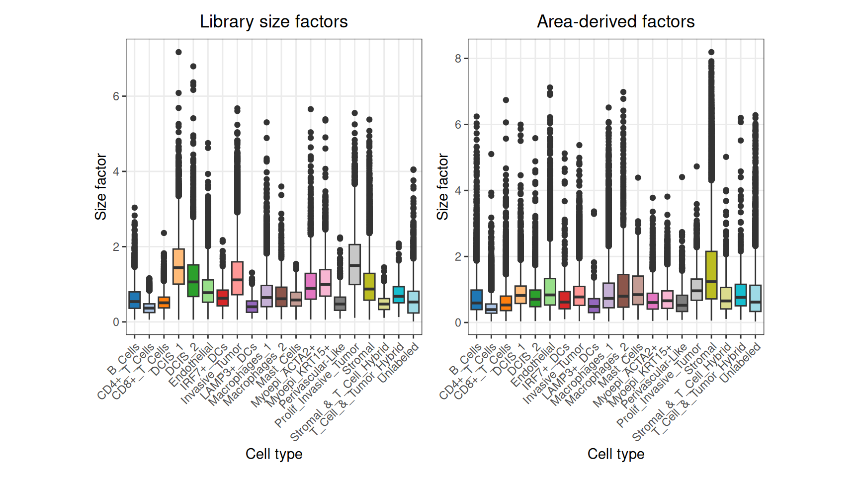
We can clearly see that library size factors of tumor cells are systematically higher than those of other cell types, which is a sign of confounding between library size and biology.

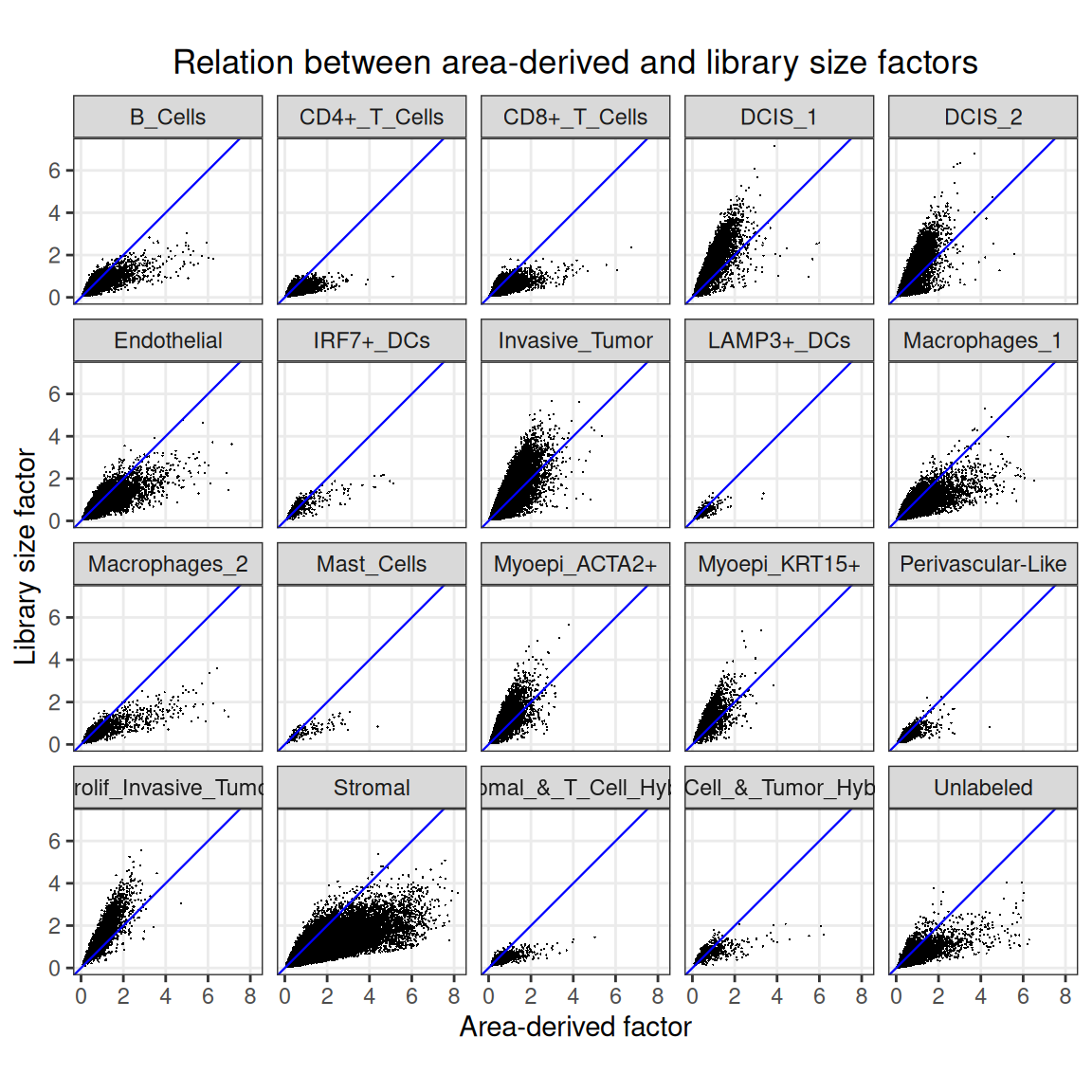
We can also compare the area-derived scaling factors with the library size factors:

ggplot(df, aes(sf_area, sf_lib)) + 
    geom_point(shape=16, stroke=0, size=0.4) +
    geom_abline(linewidth=0.4, col="blue") + 
    facet_wrap(~Label) +
    labs(x="Area-derived factor", y="Library size factor") + 
    ggtitle("Relation between area-derived and library size factors") +
    coord_equal() + theme_bw() + theme(
        panel.grid.minor=element_blank(),
        plot.title=element_text(hjust=0.5))

While there is a general correlation between total counts and cell area, the relationship is cell-type specific, with tumor cells showing systematically higher counts for a given area, and stromal cells showing generally larger areas.

This suggests that the choice of normalization may have a significant impact on downstream analyses, and should be carefully considered in the context of the specific dataset and biological questions at hand.

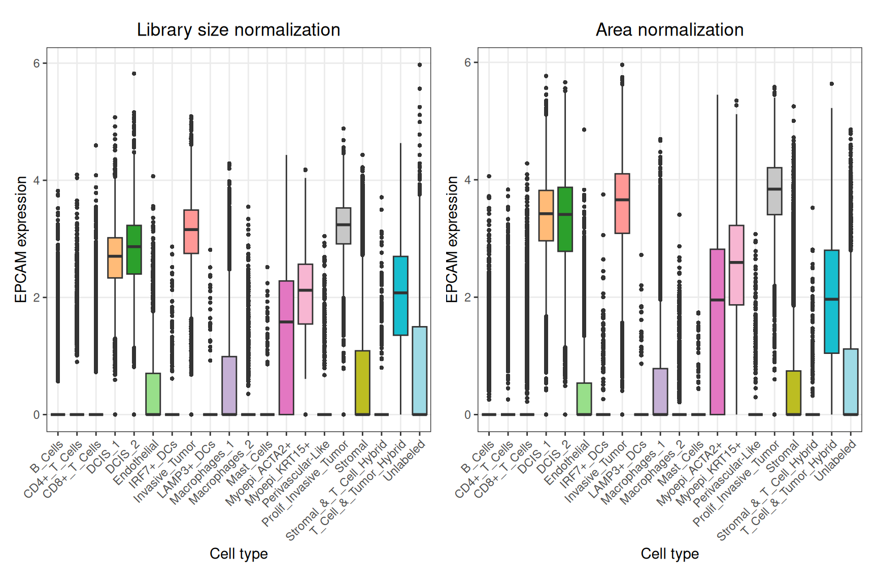
We next look at the difference in normalized expression values between the two normalization methods, and select the top 10 genes that show the largest differences.

mean_libs <- rowMeans(assays(spe)$logcounts)
mean_area <- rowMeans(assays(spe)$normalized_by_area)
diff <- abs(mean_libs - mean_area)
ord <- order(diff, decreasing=TRUE)
top_diff <- diff[ord[1:10]]
names(top_diff)

##   [1] "EPCAM"   "KRT8"    "TACSTD2" "KRT7"    "GATA3"   "CD9"     "MLPH"   
##   [8] "FASN"    "CDH1"    "FOXA1"

By looking at the top genes, we can see several epithelial cell markers, such as EPCAM, KRT8, and KRT7.

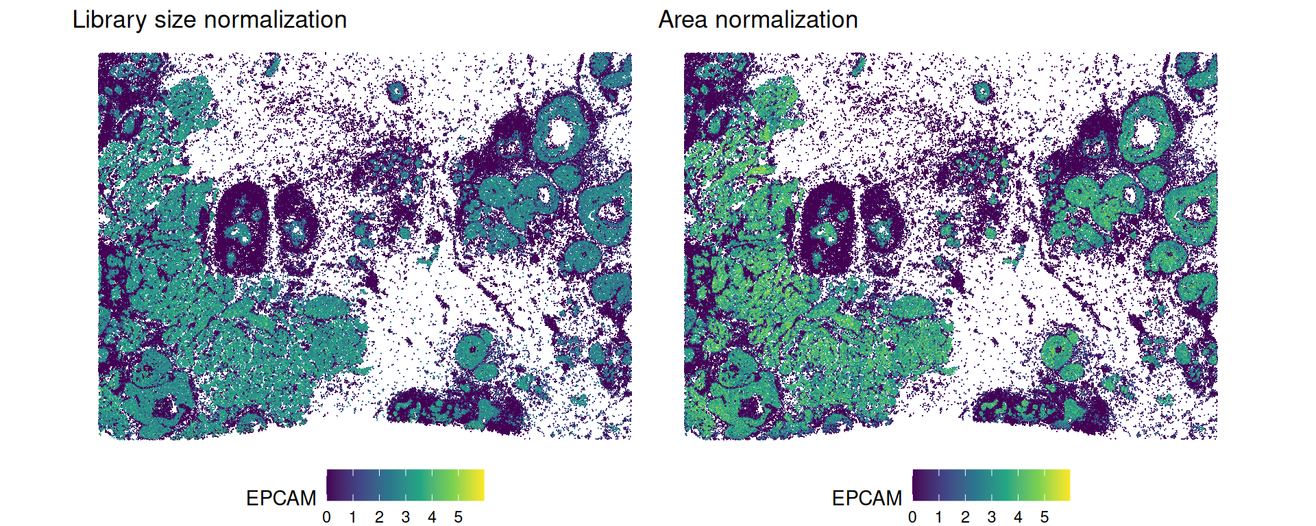
Interestingly, looking at the expression of EPCAM across the tissue, we can see that area normalization enhances the contrast between tumor and non-tumor regions, while library size normalization yields a more diffuse expression pattern.

cd <- data.frame(colData(spe), spatialCoords(spe))

mx <- logcounts(spe)[ord[1:10], ]
df_ls <- cbind(cd, as.matrix(t(mx)))

mx <- assay(spe, "normalized_by_area")[ord[1:10], ]
df_area <- cbind(cd, as.matrix(t(mx)))

p1 <- ggplot(df_ls) + labs(title="Library size normalization")
p2 <- ggplot(df_area) + labs(title="Area normalization") 

(p1 + p2) & 
    geom_point(
        aes(x_centroid, y_centroid, col=EPCAM), 
        shape=16, stroke=0, size=0.4) &
    scale_color_viridis_c() & coord_equal() & 
    theme_void() & theme(legend.position="bottom")

This is even clearer when looking at the expression of EPCAM stratified by cell type.

(p1 + p2) &
    geom_boxplot(
        aes(Label, EPCAM, fill=Label), 
        outlier.shape=16, outlier.stroke=0) &
    scale_fill_manual(values=unname(pals::tableau20())) &
    labs(x="Cell type", y="EPCAM expression") &
    theme_bw() & theme(
        aspect.ratio=1,
        legend.position="none",
        panel.grid.minor=element_blank(),
        plot.title=element_text(hjust=0.5),
        axis.text.x=element_text(angle=45, hjust=1))

27.3 Spatially-aware normalization

SpaNorm (Salim et al. 2025) is a spatially-aware normalization method that uses spatial information alongside gene expression to decompose spatially-smoothed variation into a technical and biological component. Using generalized linear models and percentile-invariant adjusted counts, SpaNorm provides normalized expression values for downstream analyses.

Given the high computational cost of SpaNorm, we do not run it here; we refer to the package vignette for details.

27.4 Appendix

TipFurther reading

• Atta et al. (2024) and Bhuva et al. (2024) highlight normalization as a key challenge in ST: library size–based methods can distort biological signal and downstream analyses, motivating alternative normalization strategies.

• Vallejos et al. (2017) highlight why assumptions underlying standard bulk RNA-seq normalization methods (e.g., consistent expression distributions, low sparsity/zero inflation) are often violated in scRNA-seq data.

• Ahlmann-Eltze and Huber (2023) compare transformations for scRNA-seq data, including variance-stabilizing approaches (delta method- and residual-based), latent expression models, and count-based factor analysis, and evaluate their impact on downstream analyses such as PCA clustering, and differential expression.

• The OSCA chapter on normalization for scRNA-seq data covers library size and spike-ins normalization, scaling and log-transformation, with practical code examples and discussion of their motivation and implications for downstream analyses.

References

Ahlmann-Eltze, Constantin, and Wolfgang Huber. 2023. “Comparison of transformations for single-cell RNA-seq data.” Nature Methods 20 (5): 665–72. https://doi.org/10.1038/s41592-023-01814-1.

Atta, Lyla, Kalen Clifton, Manjari Anant, Gohta Aihara, and Jean Fan. 2024. “Gene Count Normalization in Single-Cell Imaging-Based Spatially Resolved Transcriptomics.” Genome Biology 25 (153). https://doi.org/10.1186/s13059-024-03303-w.

Bhuva, Dharmesh D., Chin Wee Tan, Agus Salim, et al. 2024. “Library Size Confounds Biology in Spatial Transcriptomics Data.” Genome Biology 25 (99). https://doi.org/10.1186/s13059-024-03241-7.

Lun, Aaron T. L., Davis J. McCarthy, and John C. Marioni. 2016. “A Step-by-Step Workflow for Low-Level Analysis of Single-Cell RNA-Seq Data with Bioconductor.” F1000Research 5 (2122). https://doi.org/10.12688/f1000research.9501.2.

Salim, Agus, Dharmesh D. Bhuva, Carissa Chen, et al. 2025. “SpaNorm: Spatially-Aware Normalization for Spatial Transcriptomics Data.” Genome Biology 26 (109). https://doi.org/10.1186/s13059-025-03565-y.

Vallejos, Catalina A, Davide Risso, Antonio Scialdone, Sandrine Dudoit, and John C Marioni. 2017. “Normalizing single-cell RNA sequencing data: challenges and opportunities.” Nature Methods 14 (6): 565–71. https://doi.org/10.1038/nmeth.4292.