24 Subcellular analysis
24.1 Preamble
24.1.1 Introduction
Subcellular analysis aims to identify intra-cellular compartmentalization of transcripts, e.g., in the nucleus vs cytoplasm of the cell. Subcellular data can capture real biology, and analysis of subcellular data could help identify biological mechanisms involved in transcript localization (Cassella and Ephrussi 2022). Variation in intra-cellular localization of transcripts generates gene expression gradients within the cell that can affect biological processes, such as cell communication and post-transcriptional regulation.
24.1.2 Data structure
In spatially-resolved transcriptomics (SRT), subcellular analysis can be performed with molecule-resolved data generated by imaging-based SRT technologies, such as MERFISH and Xenium, where targeted probes are used to capture specific transcripts and their locations. High-resolution sequencing-based SRT data, such as Visium HD, have also been employed for subcellular analysis (Novoselsky et al. 2026).
Cell segmentation is required, prior to subcellular analysis, to generate cell boundaries within which the transcripts can be compartmentalized and assessed. MoleculeExperiment (Peters Couto et al. 2023) was built for storing transcript locations and cell boundaries, and is compatible with raw data generated by most existing molecule-resolved SRT technologies. It contains additional functions, such as countMolecules(), for conversion of molecule-resolved information to cell-level expression by counting transcripts within a cell boundary.
24.2 Quantifying cell compartments
24.2.1 Nucleus versus cell
Many molecule-resolved SRT technologies, such as MERFISH, SeqFISH, Stereo-seq, etc., provide nucleus and cell level data, generally using DAPI images to generate nuclear masks. These masks can be used to identify transcripts present in the nucleus vs cytoplasm of a cell, and the subcellular data can be used to ask a number of research questions. For example, the transport dynamics (from nucleus to cytoplasm) and localization of transcripts within cells, the impact of subcellular localization of transcripts on cell function, and comparison of subcellular location of transcripts between cells from different conditions.
24.2.2 Bento
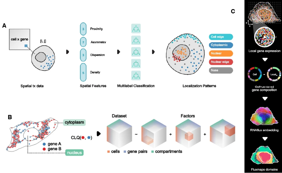
bento-tools (Mah et al. 2024) is a Python-based toolkit for subcellular analysis of molecule-resolved SRT data that takes transcript locations and boundaries (cell, nucleus, region of interest) as input and stores them in AnnData format for downstream analyses. Bento includes 3 main approaches for processing molecule-resolved data:
It generates spatial summary statistics for each gene-cell pair and feeds these into RNAforest model to predict transcript localization pattern (cytoplasmic, nuclear, nuclear edge, cell edge, or none) in each cell.
It identifies transcript compartment (nucleus or cytoplasm) from nucleus and cell boundaries, generating a cell x gene x compartment tensor. RNAcoloc approach is then applied to use the tensor for assessing colocalization of gene pairs in each compartment.
It generates RNAflux embeddings of local neighborhoods in each cell, which are used for unsupervised segmentation of subcellular domains.
These approaches supplement other downstream analyses, such as differential expression analysis between compartments or subcellular domains or enrichment analysis of these compartments/domains.
24.2.3 SpatialFeatures
SpatialFeatures is an R package that uses MoleculeExperiment to store transcript location and boundaries (cells, nuclei, and/or regions of interest), and perform subcellular and extra-cellular analyses. A SpatialFeatures run involves 3 main steps:
- Generate new subcellular (sub-concentric, sub-sector) and extra-cellular (super-concentric, super-sector) boundaries (
loadBoundaries()).
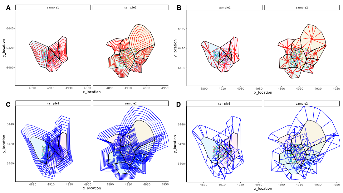
Calculate entropy-based metrics (
EntropyMatrix()) for each cell across the boundary feature type.Combine these information into a
SingleCellExperimentobject (EntropySingleCellExperiment()) containing a cell x feature matrix assay for each boundary feature type (sub-concentric, sub-sector, super-concentric, super-sector).
These features can be used to cluster and identify cells with similar subcellular and/or extra-cellular expression patterns.
24.3 Factor modeling
24.3.1 FISHFactor
FISHFactor (Walter et al. 2023) is another Python-based method for subcellular data analysis. It uses spatial Poisson point processes to model location of each transcript within each cell and spatially-aware Gaussian processes to identify subcellular localization patterns.
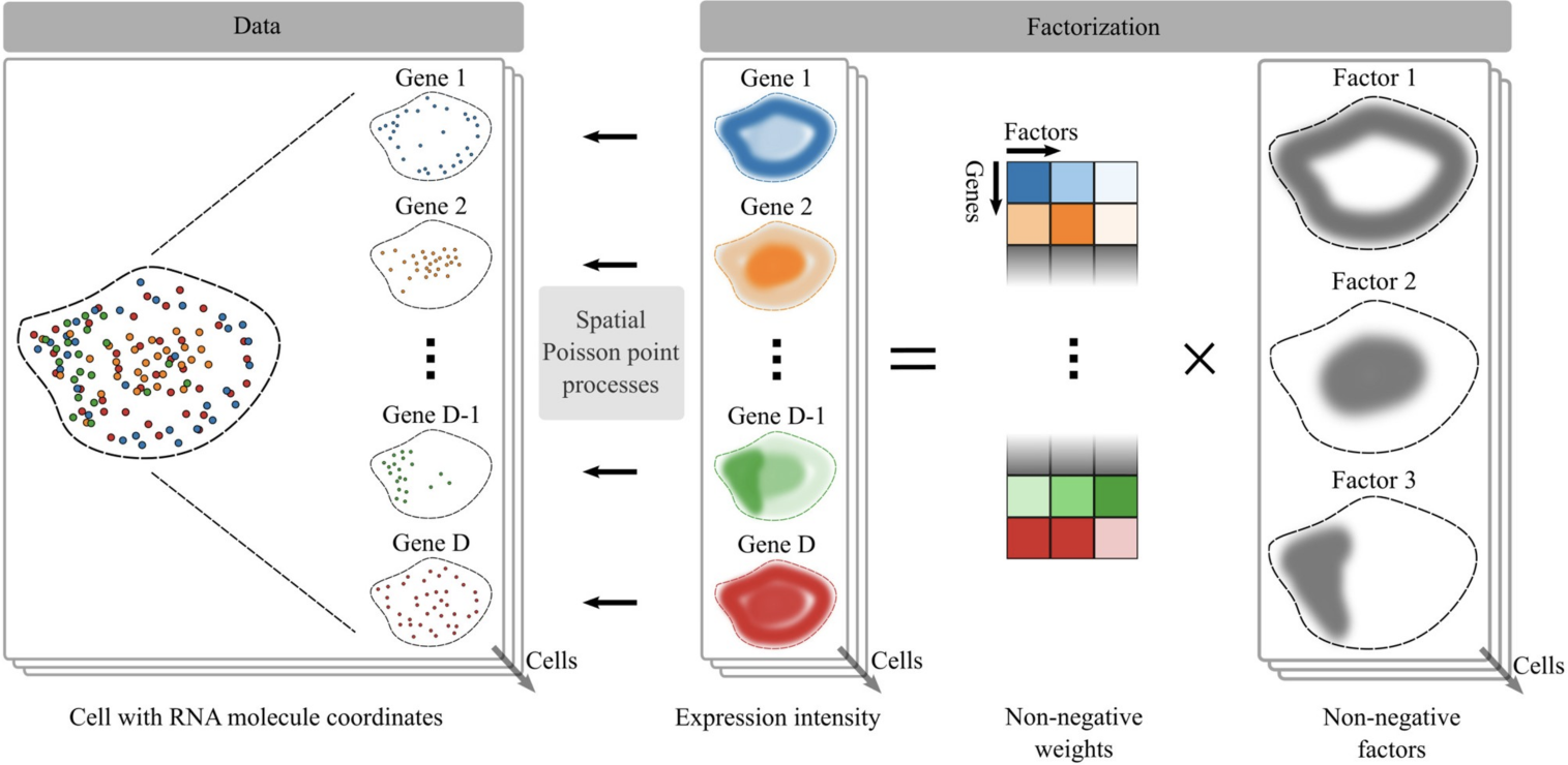
This approach focuses on transcript subcellular patterns or domains, which can be investigated further to gain biological insights (Walter et al. 2023).
24.4 Subcellular clustering
24.4.1 ClusterMap
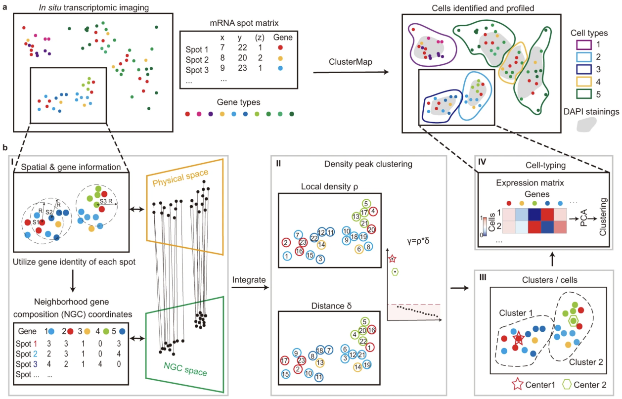
ClusterMap (He et al. 2021) is a Python-based method capable of segmentation-free spatial clustering of transcripts to multiple scales, thereby identifying subcellular domains that might represent subcellular structures or cell bodies or cell-level clusters representing cell types and domains. It can also perform cell segmentation and subcellular compartmentalization using just transcript locations. Depending on the radius used to measure neighborhood size around a transcript, it can identify clusters at subcellular (subcellular domains/compartments), cell (cell types), or tissue (domain) level, and perform subcellular or cell segmentation.
24.5 Testing for subcellular localization and colocalization
24.5.1 CellSP
CellSP (Aggarwal and Sinha 2025) is a Python-based workflow for identifying subcellular patterns of transcripts that can be further used to identify and characterize gene-cell modules. It provides tools for visualizing the gene-cell modules and examining their functional significance.
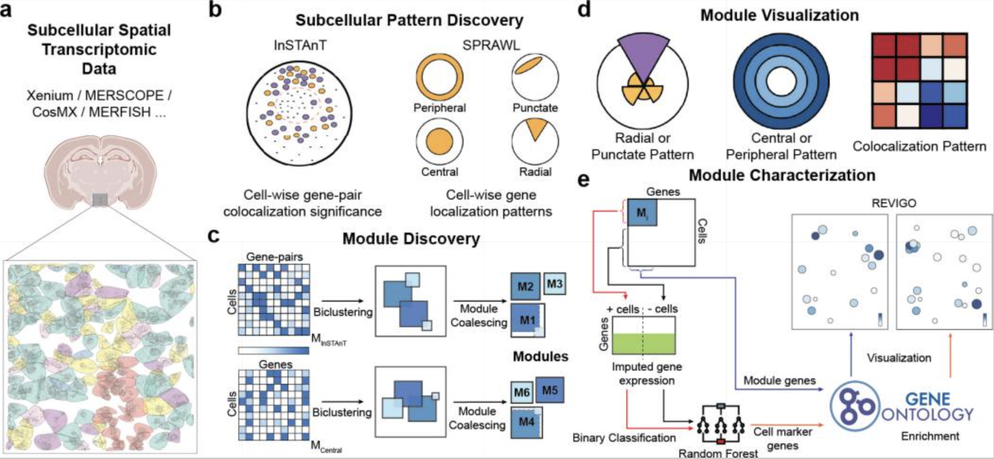
CellSP uses AnnData format for single cell and spatial transcriptomics analysis. Internally, CellSP uses other tools, such as MAGIC (Dijk et al. 2018) for denoising, Tangram (Biancalani et al. 2021) for imputation, InSTAnT (Kumar et al. 2024) for identifying gene-pair subcellular colocalization patterns, and SPRAWL (Bierman et al. 2024) for identifying gene subcellular localization patterns.
CellSP outputs a set of gene-cell modules for each subcellular pattern type (peripheral, radial, punctate, central, colocalization). A gene-cell module represents a set of genes or gene pairs that have the same subcellular pattern across the same set of cells. The statistical significance of grouping is estimated using a Bonferroni-based score. In each module, genes and cells are characterized using gene ontology (GO) enrichment tests and cell type composition (if available), respectively.
Some statistical tests for gene(s) localization/colocalization that can be performed using CellSP include:
Testing per cell – does a cell have significant subcellular localization of a set of genes or gene-pairs?
Testing across multiple cells – do cells belonging to a cell type/cluster have significant subcellular localization of a gene or gene pair?
Testing across multiple groups/samples – are specific genes differentially localized/colocalized in two cell types/clusters from one sample or a cell type/cluster from two different conditions?
24.5.2 SpaGNN
spaGNN (Fang et al. 2023) is another Python-based pipeline for subcellular analyses, including:
Subcellular clustering of transcript locations into subcellular patches with high transcript density using Leiden graph clustering.
Subcellular patch analysis, where transcripts of each gene in each patch are summed to generate a patch-by-gene count matrix. This is used to calculate Pearson’s correlation between genes across all patches, to identify gene pairs that often colocalize. The statistical significance of these correlation values can be assessed using a t-test.
Subcellular local neighborhoods are detected within a patch by identifying 9 nearest neighbors of each transcript in the patch. Further analysis involves summing transcript counts in the local neighborhoods and calculating Pearson’s correlation between genes. Through permutation analysis, a proximity score is calculated for each gene pair in the patch.
Depending on availability of cell type data, additional questions can be asked. For example, how similar are the patch correlations between same/different cell types, or how consistent is the subcellular colocalization of a gene pair in same/different cell types?
24.6 Considerations
24.6.1 2D versus 3D
A majority of the molecule-resolved SRT data are 2D projections of 3D structures, such as cells, organelles, or even processes like RNA transport. A few imaging-based SRT technologies are capable of measuring tissue depth as z-axis, generating 3D coordinates with a sparse z-axis. However, working with 2D versus 3D data is not so different, since spatial relations are often captured as neighborhoods defined by Euclidean or other distance measures between locations, irrespective of coordinate dimension. Therefore, many tools are able to use n-dimensional coordinates for measuring spatial relationships. For example, ClusterMap can use 3D coordinates by using z_radius for z-axis data, if it’s available, whereas for 2D coordinates it sets z_radius = 0 (He et al. 2021).
24.7 Appendix
References
Aggarwal, Bhavay, and Saurabh Sinha. 2025. “CellSP: Module Discovery and Visualization for Subcellular Spatial Transcriptomics Data.” bioRxiv, ahead of print. https://doi.org/10.1101/2025.01.12.632553.
Biancalani, Tommaso, Gabriele Scalia, Lorenzo Buffoni, et al. 2021. “Deep Learning and Alignment of Spatially Resolved Single-Cell Transcriptomes with Tangram.” Nature Methods 18: 1352–62. https://doi.org/10.1038/s41592-021-01264-7.
Bierman, Rob, Jui M Dave, Daniel M Greif, and Julia Salzman. 2024. “Statistical Analysis Supports Pervasive RNA Subcellular Localization and Alternative 3’ UTR Regulation.” eLife 12. https://doi.org/10.7554/elife.87517.
Cassella, Lucia, and Anne Ephrussi. 2022. “Subcellular Spatial Transcriptomics Identifies Three Mechanistically Different Classes of Localizing RNAs.” Nature Communications 13 (1). https://doi.org/10.1038/s41467-022-34004-2.
Dijk, David van, Roshan Sharma, Juozas Nainys, et al. 2018. “Recovering Gene Interactions from Single-Cell Data Using Data Diffusion.” Cell 174 (3): 716–729.e27. https://doi.org/10.1016/j.cell.2018.05.061.
Fang, Zhou, Adam J. Ford, Thomas Hu, Nicholas Zhang, Athanasios Mantalaris, and Ahmet F. Coskun. 2023. “Subcellular Spatially Resolved Gene Neighborhood Networks in Single Cells.” Cell Reports Methods 3 (5): 100476. https://doi.org/10.1016/j.crmeth.2023.100476.
He, Yichun, Xin Tang, Jiahao Huang, et al. 2021. “ClusterMap for Multi-Scale Clustering Analysis of Spatial Gene Expression.” Nature Communications 12 (1). https://doi.org/10.1038/s41467-021-26044-x.
Kumar, Anurendra, Alex W. Schrader, Bhavay Aggarwal, et al. 2024. “Intracellular Spatial Transcriptomic Analysis Toolkit (InSTAnT).” Nature Communications 15 (1). https://doi.org/10.1038/s41467-024-49457-w.
Mah, Clarence K., Noorsher Ahmed, Nicole A. Lopez, et al. 2024. “Bento: A Toolkit for Subcellular Analysis of Spatial Transcriptomics Data.” Genome Biology 25 (1). https://doi.org/10.1186/s13059-024-03217-7.
Novoselsky, Roy, Ofra Golani, Tal Barkai, et al. 2026. “Subcellular mRNA localization patterns across tissues resolved with spatial transcriptomics.” Nature Communications, 1–13. https://doi.org/10.1038/s41467-026-72156-7.
Peters Couto, Bárbara Zita, Nicholas Robertson, Ellis Patrick, and Shila Ghazanfar. 2023. “MoleculeExperiment Enables Consistent Infrastructure for Molecule-Resolved Spatial Omics Data in Bioconductor.” Bioinformatics 39 (btad550, 9). https://doi.org/10.1093/bioinformatics/btad550.
Walter, Florin C, Oliver Stegle, and Britta Velten. 2023. “FISHFactor: A Probabilistic Factor Model for Spatial Transcriptomics Data with Subcellular Resolution.” Bioinformatics 39 (5). https://doi.org/10.1093/bioinformatics/btad183.