13 Deconvolution
13.1 Preamble
13.1.1 Introduction
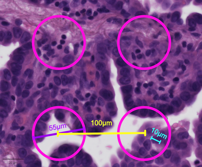
Sequencing-based ST data can contain zero to multiple cells per spot, which might be fully or only partially covered by cells, depending on the spatial resolution of the platform and the tissue cell density (see also Chapter 9 and the schematic Figure below). This aspect of the data implies that there may be a mixture of cell types in a spot and thus a mixture of transcriptional programs.
To help understand these mixtures, at least 20 deconvolution techniques have been proposed for spot-level ST data. Some methods require borrowing insights from a scRNA-seq reference dataset, while others can be reference-free. Based on their underlying algorithms, Li et al. (2023) have grouped methods into five categories:
-
probabilistic-based: use Bayesian inference, likelihood estimation, or probabilistic modeling to estimate cell type compositions while incorporating uncertainty. Available tools include
- CARDspa (Ma and Zhou 2022)
-
spacexr’s
RCTD(Cable et al. 2022) - SpatialDecon (Danaher et al. 2022)
- STdeconvolve (Miller et al. 2022) in R, and
- cell2location (Kleshchevnikov et al. 2022)
-
scvi-tools’s
DestVI(Lopez et al. 2022) - std-poisson (Berglund et al. 2018)
- stereoscope (Andersson et al. 2020)
- STRIDE (Sun et al. 2022) in Python.
non-negative matrix factorization (NMF)-based: decompose gene expression data into latent components representing different cell types. Available tools include Giotto’s
SpatialDWLS(Chen et al. 2025) and SPOTlight (Elosua-Bayes et al. 2021) in R, and NMFreg_tutorial in Python.graph-based: use graph neural networks or graph-based optimization to model spatial relationships. Available tools include SD2 (Li et al. 2022) in R, and DSTG (Song and Su 2021) and SpiceMIx (Chidester et al. 2023) in Python.
optimal transport (OT)-based: infer spatial gene expression distributions by mapping scRNA-seq and ST data. Available tools include SpaOTsc (Cang and Nie 2020) and novosparc (Nitzan et al. 2019) in Python.
deep learning-based: align and integrate single-cell and spatial transcriptomics data with neural networks. For example, Tangram (Biancalani et al. 2021) in Python.
Among these, std-poisson, STdeconvolve, and SpiceMix are reference-free methods. Methods that incorporate spatial location information are CARD, DSTG, SD2, Tangram, cell2location, DestVI, std-poisson, and SpiceMix.
In this chapter, we demonstrate deconvolution of cell types per spot, using RCTD on Visium and Visium HD datasets. For related examples where deconvolution is one step within a broader workflow, see Chapter 15 and Chapter 16.
13.1.2 Dependencies
In this example of Visium breast cancer data (Janesick et al. 2023), we perform cell type deconvolution without a single-cell (Chromium) reference and compare the concordance with the Visium annotation provided by 10x Genomics.
Code
# retrieve dataset from OSF repository
id <- "Visium_HumanBreast_Janesick"
pa <- OSTA.data_load(id)
dir.create(td <- tempfile())
unzip(pa, exdir=td)

# read into 'SpatialExperiment'
vis <- TENxVisium(
    spacerangerOut=file.path(td, "outs"),
    processing="filtered",
    format="h5",
    images="lowres") |>
    import()

# retrieve spot annotations & add as metadata
df <- read.csv(file.path(td, "annotation.csv"))
cs <- match(colnames(vis), df$Barcode)
vis$anno <- factor(df$Annotation[cs])

# set gene symbols as feature names
rownames(vis) <- make.unique(rowData(vis)$Symbol)
vis
## class: SpatialExperiment
## dim: 18085 4992
## metadata(2): resources spatialList
## assays(1): counts
## rownames(18085): SAMD11 NOC2L ... MT-ND6 MT-CYB
## rowData names(3): ID Symbol Type
## colnames(4992): AACACCTACTATCGAA-1 AACACGTGCATCGCAC-1 ...
## TGTTGGCCAGACCTAC-1 TGTTGGCCTACACGTG-1
## colData names(5): in_tissue array_row array_col sample_id anno
## reducedDimNames(0):
## mainExpName: Gene Expression
## altExpNames(0):
## spatialCoords names(2) : pxl_col_in_fullres pxl_row_in_fullres
## imgData names(4): sample_id image_id data scaleFactorCode
xy <- spatialCoords(vis) * scaleFactors(vis)
ys <- nrow(imgRaster(vis)) - range(xy[, 2])
xs <- range(xy[, 1])
box <- geom_rect(
    xmin=xs[1], xmax=xs[2], ymin=ys[1], ymax=ys[2],
    col="black", fill=NA, linetype=2, linewidth=2/3)
plotVisium(vis, spots=FALSE, point_size=1) + box +
    plotVisium(vis, point_size=1, zoom=TRUE) +
    plot_layout(nrow=1) & facet_null()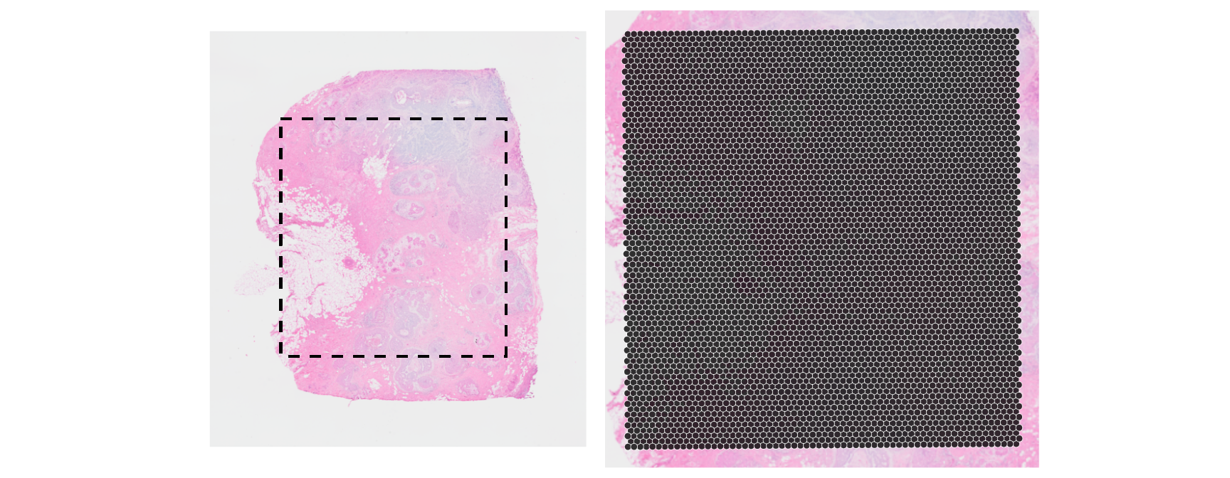
Deconvolution is performed after quality control, as detailed in Chapter 11, and is usually performed on unnormalized and untransformed (i.e. raw) counts. Here, we quickly check some typically spot-level metrics.
Code
sub <- list(mt=grepl("^MT-", rownames(vis)))
vis <- quickRnaQc.se(vis, subsets=sub)
Code
vis$log_sum <- log1p(vis$sum)
plotCoords(vis,
    annotate="log_sum") +
    ggtitle("log library size") +
plotCoords(vis,
    annotate="subset.proportion.mt") +
    ggtitle("mitochondrial fraction") +
ggplot(
    data.frame(colData(vis)),
    aes(x=sum, y=subset.proportion.mt)) +
    geom_point() + geom_density_2d() +
    scale_x_log10() + scale_y_sqrt() +
    theme(aspect.ratio=2/3) +
plot_layout(nrow=1) & theme(
    legend.key.width=unit(0.5, "lines"),
    legend.key.height=unit(1, "lines")) &
    scale_color_gradientn(colors=pals::jet())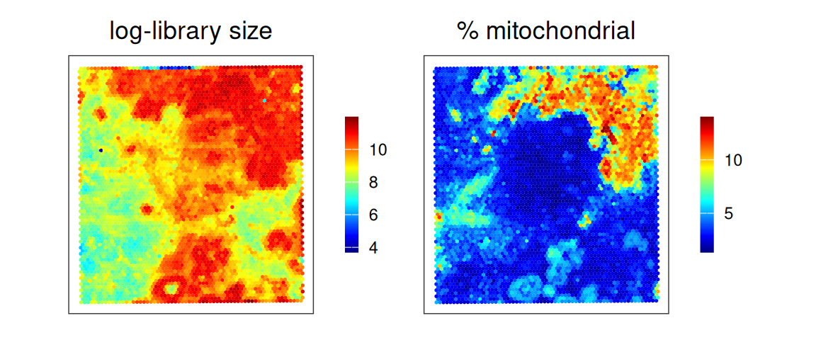
A few spots have low library sizes, and can be removed.
Code
vis <- vis[, vis$sum > 1000]We first visualize the spot-level cell type annotation provided by 10x Genomics.
Code
plotCoords(vis,
    annotate="anno", point_size=1,
    pal=unname(pals::trubetskoy())) +
    theme(legend.key.size=unit(0, "lines"))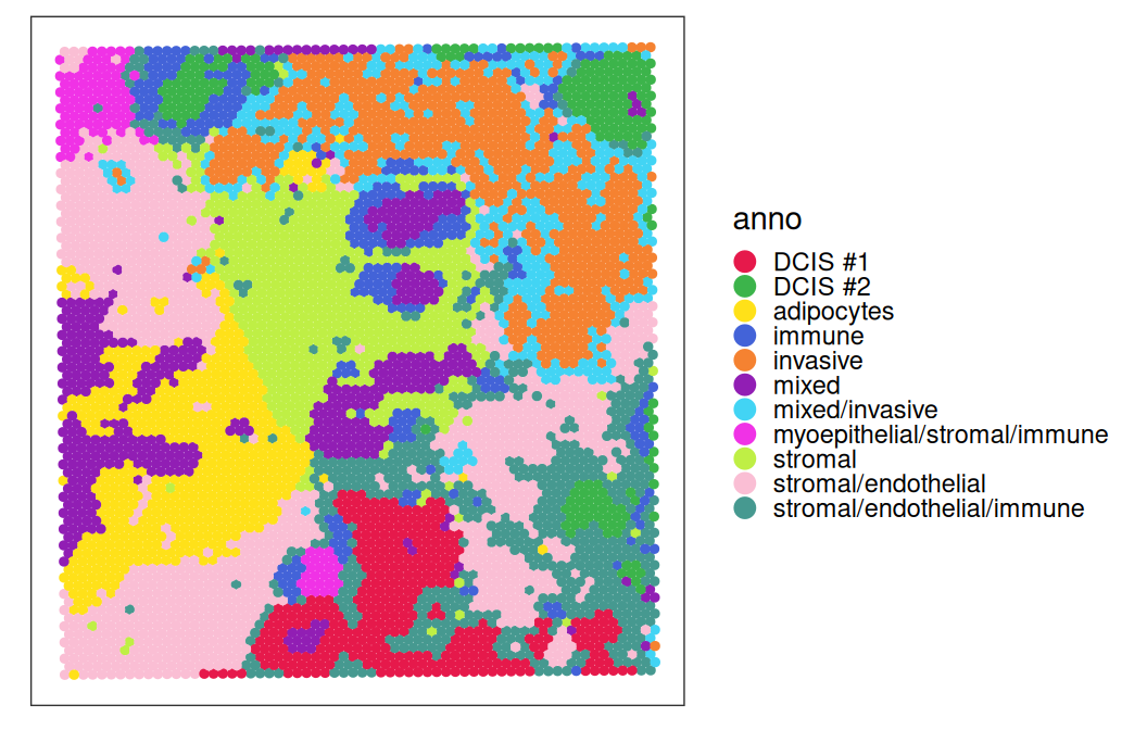
Now, we load the single-cell (Chromium) reference data for the Visium dataset. To streamline the demonstration, we consolidate some of the cell type annotations provided by 10x Genomics (i.e. Annotation) into more generalized categories (i.e. Annogrp).
Code
# retrieve dataset from OSF repo
id <- "Chromium_HumanBreast_Janesick"
pa <- OSTA.data_load(id)
dir.create(td <- tempfile())
unzip(pa, exdir=td)

# read into 'SingleCellExperiment'
fs <- list.files(td, full.names=TRUE)
h5 <- grep("h5$", fs, value=TRUE)
sce <- read10xCounts(h5, col.names=TRUE)

# use gene symbols as feature names
rownames(sce) <- make.unique(rowData(sce)$Symbol)

# retrieve cell type labels
csv <- grep("csv$", fs, value=TRUE)
cd <- read.csv(csv, row.names=1)

# ignore mixtures
lab <- cd$Annotation
lab[grepl("Hyb", lab)] <- NA

# simplify annotations
pat <- c(
    "B Cell"="B", "T Cell"="T", "Mac"="macro", "Mast"="mast",
    "DCs"="dendritic", "Peri"="perivas", "End"="endo",
    "Str"="stromal", "Inv"="tumor", "Myo"="myoepi")
for (. in names(pat))
    lab[grep(., lab)] <- pat[.]
lab <- gsub("\\s", "", lab)

# add as cell metadata
table(cd$Annogrp <- lab)
##
## B DCIS1 DCIS2 T dendritic endo macro
## 1463 1863 2159 4742 313 1055 3724
## mast myoepi perivas stromal tumor
## 92 1839 285 2611 5897We only keep the Chromium data with an annotation and are not labeled as “Hybrid”, as these correspond to mixed subpopulations.
13.2 RCTD
Next, we perform deconvolution with spacexr (also known as RCTD) (Cable et al. 2022). By default, runRctd()’s rctd_mode = "doublet" specifies at most two subpopulations coexist in a data unit (i.e. within a spot); here, we set rctd_mode = "full" in order to allow for an arbitrary number of subpopulations to be fit instead.
Note that RCTD can also be adapted to Visium HD data with
rctd_mode = "doublet", as demonstrated by (de Oliveira et al. 2025) and Chapter 17.Code
rctd_data <- createRctd(vis, sce, cell_type_col="Annogrp")
(res <- runRctd(rctd_data, max_cores=4, rctd_mode="full"))
## class: SpatialExperiment
## dim: 12 4962
## metadata(4): spatial_rna config cell_type_info internal_vars
## assays(1): weights
## rownames(12): B DCIS1 ... stromal tumor
## rowData names(0):
## colnames(4962): AACACCTACTATCGAA-1 AACACGTGCATCGCAC-1 ...
## TGTTGGCCAGACCTAC-1 TGTTGGCCTACACGTG-1
## colData names(1): sample_id
## reducedDimNames(0):
## mainExpName: NULL
## altExpNames(0):
## spatialCoords names(2) : x y
## imgData names(0):Weights inferred by RCTD should be normalized such that proportions of cell types sum to 1 for each spot:
Code
##                        B DCIS1 DCIS2    T dendritic
##  AACACCTACTATCGAA-1 0.00  0.00  0.00 0.00      0.01
##  AACACGTGCATCGCAC-1 0.04  0.01  0.00 0.04      0.00
##  AACACTTGGCAAGGAA-1 0.00  0.00  0.03 0.01      0.01
##  AACAGGAAGAGCATAG-1 0.03  0.00  0.00 0.08      0.03
## AACAGGATTCATAGTT-1 0.00 0.00 0.01 0.00 0.0013.3 CARD
Another method that can be used is CARD. First, we rename the columns of spatial coordinates for CARD.
Next, we perform the CARD deconvolution. Here, we demonstrate CARD’s interoperability with SingleCellExperiment and SpatialExperiment. The deconvolution result matrix is already normalized such that the sum of cell type proportions for each spot is equal to 1.
Note:
CARD can also take a reference matrix, a reference cell type annotation column, a spatial count matrix, and a spatial coordinates data frame as separate items in sc_count, sc_meta, spatial_count, and spatial_location, respectively. However, we encourage simplifying the process by using existing Bioconductor classes.Code
set.seed(2025)
CARD_obj <- CARD_deconvolution(
    spe=vis,
    sce=sce,
    sc_count=NULL,
    sc_meta=NULL,
    spatial_count=NULL,
    spatial_location=NULL,
    ct_varname="Annogrp",
    ct_select=NULL,      # use all 'sce$Annogrp' cell types
    sample_varname=NULL, # use all 'sce' as one 'ref' sample
    mincountgene=100,
    mincountspot=5)
ws_card <- CARD_obj$Proportion_CARD

# order cell type names alphabetically, as for RCTD
ws_card <- data.frame(ws_card[, colnames(ws_rctd)])
round(ws_card[1:5, 1:5], 2)
## B DCIS1 DCIS2 T dendritic
## AACACCTACTATCGAA-1 0 0 0 0.00 0
## AACACGTGCATCGCAC-1 0 0 0 0.00 0
## AACACTTGGCAAGGAA-1 0 0 0 0.01 0
## AACAGGAAGAGCATAG-1 0 0 0 0.02 0
## AACAGGATTCATAGTT-1 0 0 0 0.00 013.4 Visualization
First, we define a couple accessory functions.
Code
.plt_xy <- \(ws, vis, col, point_size) {
    xy <- spatialCoords(vis)[rownames(ws), ]
    colnames(xy) <- c("x", "y")
    df <- cbind(ws, xy)
    ggplot(df, aes(x, y, col=.data[[col]])) +
        coord_equal() + theme_void() +
        geom_point(size=point_size)
}

.plt_decon <- \(ws, vis) {
    ps <- lapply(names(ws), \(.) .plt_xy(ws, vis, col=., point_size=0.3))
    ps |> wrap_plots(nrow=3) & theme(
        legend.key.width=unit(0.5, "lines"),
        legend.key.height=unit(1, "lines")) &
        scale_color_gradientn(colors=pals::jet())
}
We can visualize deconvolution weights in x-y space, i.e., coloring by the proportion of a given cell type estimated to fall within a given spot:
Code
.plt_decon(ws=ws_rctd, vis)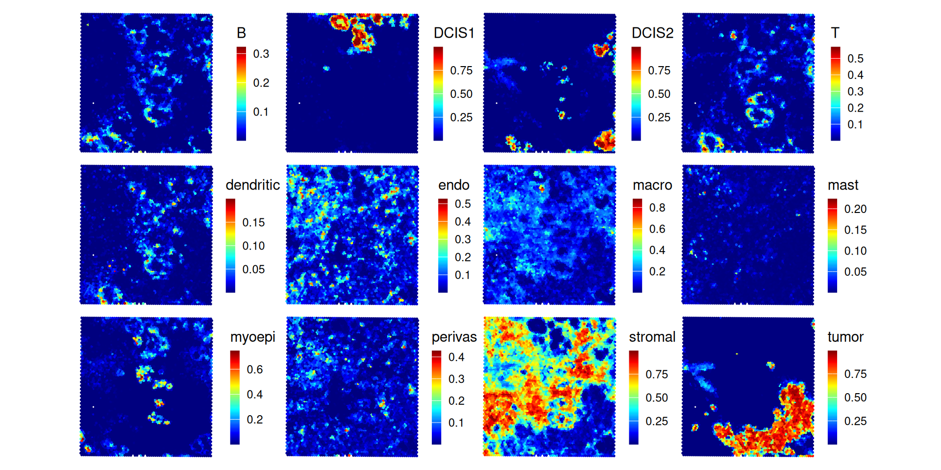
Code
.plt_decon(ws=ws_card, vis)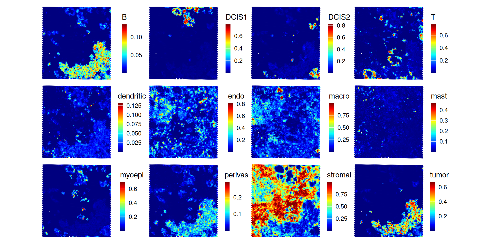
The deconvolution results can also be viewed as a heatmap, where rows = cells and columns = clusters:
Code
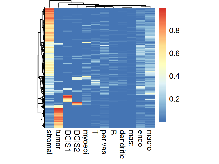
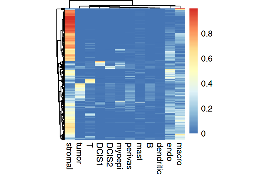
In both methods, we see that more than half of the spots are estimated to have a stromal proportion of more than 50%. Few spots have an intense and distinct signal for cancerous subpopulations, DCIS1 and DCIS2. For the following analysis, we focus on RCTD as an example.
For comparison with spot annotations provided by 10x Genomics, we include majority voted cell type from deconvolution by RCTD. Note that, because stromal cells show broad signals across the entire tissue, to better investigate immune cell signals, we remove stromal from the majority vote calculation for an alternative label: RCTD_no_stroma.
Code
ws <- ws_rctd
# derive majority vote label
ids <- names(ws)[apply(ws, 1, which.max)]
names(ids) <- rownames(ws)
vis$RCTD <- factor(ids[colnames(vis)])

# derive majority vote excluding stromal cells
ws_no_stroma <- ws[, colnames(ws) != "stromal"]
ids_no_stroma <- names(ws_no_stroma)[apply(ws_no_stroma, 1, which.max)]
names(ids_no_stroma) <- rownames(ws)
vis$RCTD_no_stroma <- factor(ids_no_stroma[colnames(vis)])
We can visualize these three annotations spatially:
Code
lapply(
    c("anno", "RCTD", "RCTD_no_stroma"),
    \(.) plotCoords(vis, annotate=.)) |>
    wrap_plots(nrow=1) &
    theme(legend.key.size=unit(0, "lines")) &
    scale_color_manual(values=unname(pals::trubetskoy()))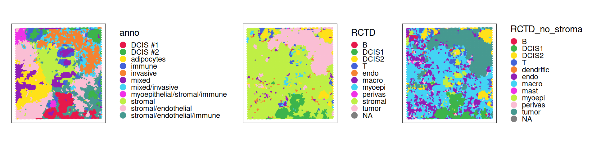
Note the strong stromal signals and macrophages being the second most common cell type for stromal cells. To help characterize subpopulations from deconvolution, we can view their distribution against the provided annotation:
Code
cd <- data.frame(colData(vis))
df <- as.data.frame(with(cd, table(RCTD, anno)))
fd <- as.data.frame(with(cd, table(RCTD_no_stroma, anno)))
ggplot(df,
    aes(Freq, RCTD, fill=anno)) +
    ggtitle("RCTD") +
ggplot(fd,
    aes(Freq, RCTD_no_stroma, fill=anno)) +
    ggtitle("RCTD_no_stroma") +
plot_layout(nrow=1, guides="collect") &
    labs(x="Proportion", y=NULL) &
    coord_cartesian(expand=FALSE) &
    geom_col(width=1, col="white", position="fill") &
    scale_fill_manual(values=unname(pals::trubetskoy())) &
    theme_minimal() & theme(
        aspect.ratio=1,
        legend.key.size=unit(2/3, "lines"),
        plot.title=element_text(hjust=0.5))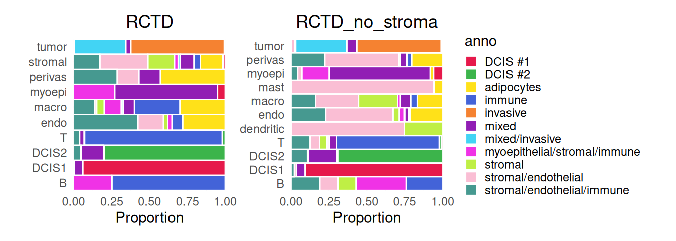
Next, we can investigate the agreement between the provided annotation against the two deconvolution majority vote labels.
Code
hm <- \(mat, string) pheatmap(
    mat, show_rownames=TRUE, show_colnames=TRUE, main=string,
    cellwidth=10, cellheight=10, treeheight_row=5, treeheight_col=5)
hm(prop.table(table(vis$anno, vis$RCTD), 2), string="RCTD")
hm(prop.table(table(vis$anno, vis$RCTD_no_stroma), 2), string="RCTD_no_stroma")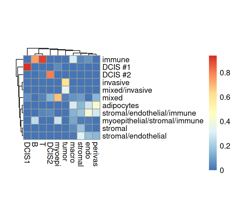
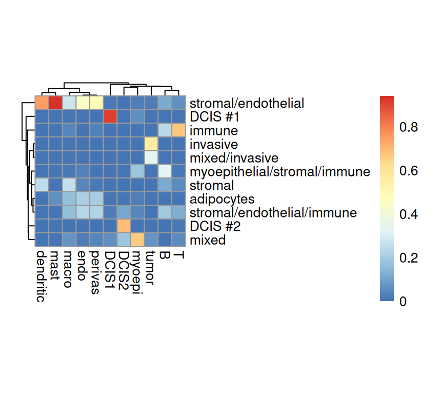
Overall, we observe agreement between the provided spot labels and the RCTD deconvolution derived annotations. Before cleaning up stromal, some immune cell types, such as dendritic and mast, never had a chance to have the highest cell type proportion. On the left panel, among all the spots annotated by RCTD as T cells, nearly all of them are from the “immune” type in the provided annotation. Strong agreements are also observed for spots with cell type of “DCIS1”, “DCIS2”, and “Invasive tumor”.
NotePC regression
Next, we prepare the principal components (PCs) needed to perform PC regression:
Code
# log-library size normalization
vis <- normalizeRnaCounts.se(vis)
# feature selection
vis <- chooseRnaHvgs.se(
    vis,
    top=ceiling(0.1 * nrow(vis)),
    more.var.args=list(use.min.width=TRUE))
hvg <- rownames(vis)[rowData(vis)$hvg]
# dimension reduction
set.seed(1234)
vis <- runPca.se(vis, features=hvg, number=20)
colnames(reducedDim(vis, "PCA")) <- paste0(
    "PC", seq_len(ncol(reducedDim(vis, "PCA"))))
We fit the deconvolution result of each cell type against the first 10 PCs to obtain 10 regressions.
Here we plot the coefficient of determination of the first 10 PCs for each cell type.
Code
pcr$id <- factor(pcr$id, ids)
pal <- pals::trubetskoy()
ggplot(pcr, aes(pc, r2, col=id)) +
    geom_line(show.legend=FALSE) + geom_point() +
    scale_color_manual("predictor", values=unname(pal)) +
    scale_x_continuous(breaks=c(1, seq(5, 20, 5))) +
    scale_y_continuous(limits=c(0, 1), breaks=seq(0, 1, 0.2)) +
    labs(x="principal component", y="coeff. of determination") +
    guides(col=guide_legend(override.aes=list(size=2))) +
    coord_cartesian(xlim=c(1, 10)) +
    theme_minimal() + theme(
      panel.grid.minor=element_blank(),
      legend.key.size=unit(0, "lines"))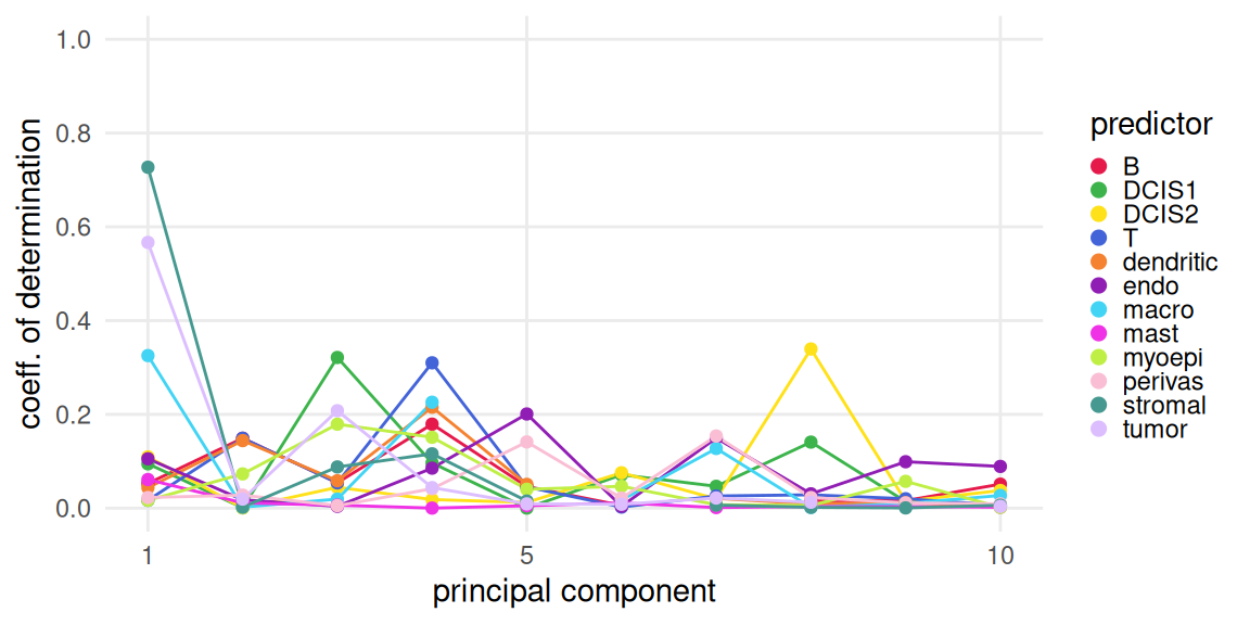
Let’s inspect the key drivers of (expression) variability in terms of PCs. Considering deconvolution results from above, we can see that, e.g.:
- PC1 distinguishes stromal, tumor, macrophage from the rest of the tissue
- PC3, PC4 and PC5 separate DCIS1, T and endothelial cells, respectively
Code
# retrieve top-10 PCs
pcs <- reducedDim(vis, "PCA")
pcs <- pcs[rownames(ws), seq_len(10)]
# specify subpopulations & PCs to visualize
var <- c("DCIS1", "T", "endo")
var <- c(var, colnames(pcs)[3:5])
# visualize deconvolution weights alongside PCs
lapply(var, \(.) {
    .plt_xy(
        cbind(ws, pcs), vis, col=., point_size=0.3) +
        scale_color_gradientn(., colors=pals::jet())
}) |>
    wrap_plots(nrow=2) & theme(
        plot.title=element_blank(),
        legend.key.width=unit(0.5, "lines"),
        legend.key.height=unit(1, "lines"))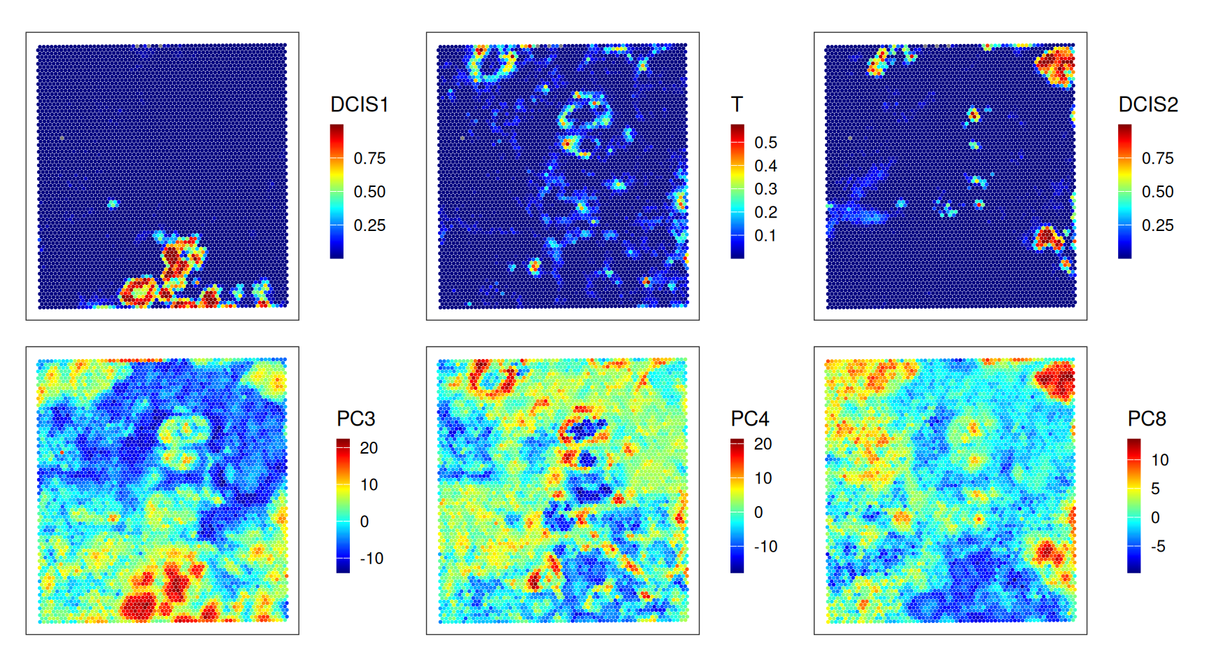
Note that the direction of each PC is irrelevant from how much variation it explains.
In conclusion, deconvolution-based cell type proportion estimates are able to recapitulate PCs and, in turn, expression variability.
Apart from being a tool for spot deconvolution,
RCTD can be used as a label transfer tool to annotate imaging-based ST data, such as for Xenium and MERSCOPE. For this, the default doublet_mode = "doublet" should be used, and a certainty score would be returned to indicate doublets with two predicted cell types.13.5 Appendix
References
Andersson, Alma, Joseph Bergenstråhle, Michaela Asp, et al. 2020. “Single-Cell and Spatial Transcriptomics Enables Probabilistic Inference of Cell Type Topography.” Communications Biology 3 (1): 565. https://doi.org/10.1038/s42003-020-01247-y.
Berglund, Emelie, Jonas Maaskola, Niklas Schultz, et al. 2018. “Spatial Maps of Prostate Cancer Transcriptomes Reveal an Unexplored Landscape of Heterogeneity.” Nature Communications 9 (1): 2419. https://doi.org/10.1038/s41467-018-04724-5.
Biancalani, Tommaso, Gabriele Scalia, Lorenzo Buffoni, et al. 2021. “Deep Learning and Alignment of Spatially Resolved Single-Cell Transcriptomes with Tangram.” Nature Methods 18: 1352–62. https://doi.org/10.1038/s41592-021-01264-7.
Cable, Dylan M., Evan Murray, Luli S. Zou, et al. 2022. “Robust Decomposition of Cell Type Mixtures in Spatial Transcriptomics.” Nature Biotechnology 40: 517–26. https://doi.org/10.1038/s41587-021-00830-w.
Cang, Zixuan, and Qing Nie. 2020. “Inferring Spatial and Signaling Relationships Between Cells from Single Cell Transcriptomic Data.” Nature Communications 11 (2084). https://doi.org/10.1038/s41467-020-15968-5.
Chen, Jiaji G, Joselyn C Chávez-Fuentes, Matthew O’Brien, et al. 2025. “Giotto Suite: A Multiscale and Technology-Agnostic Spatial Multiomics Analysis Ecosystem.” Nature Methods, 1–13. https://doi.org/10.1038/s41592-025-02817-w.
Chidester, Benjamin, Tianming Zhou, Shahul Alam, and Jian Ma. 2023. “SpiceMix Enables Integrative Single-Cell Spatial Modeling of Cell Identity.” Nat. Genet. 55 (1): 78–88. https://doi.org/10.1038/s41588-022-01256-z.
Danaher, Patrick, Youngmi Kim, Brenn Nelson, et al. 2022. “Advances in Mixed Cell Deconvolution Enable Quantification of Cell Types in Spatial Transcriptomic Data.” Nature Communications 13 (1): 385. https://doi.org/10.1038/s41467-022-28020-5.
de Oliveira, Michelli Faria, Juan Pablo Romero, Meii Chung, et al. 2025. “High-Definition Spatial Transcriptomic Profiling of Immune Cell Populations in Colorectal Cancer.” Nature Genetics 57: 1512–23. https://doi.org/10.1038/s41588-025-02193-3.
Elosua-Bayes, Marc, Paula Nieto, Elisabetta Mereu, Ivo Gut, and Holger Heyn. 2021. “SPOTlight: Seeded NMF Regression to Deconvolute Spatial Transcriptomics Spots with Single-Cell Transcriptomes.” Nucleic Acids Research 49 (9): e50. https://doi.org/10.1093/nar/gkab043.
Gaspard-Boulinc, Lucie C., Luca Gortana, Thomas Walter, Emmanuel Barillot, and Florence M. G. Cavalli. 2025. “Cell-Type Deconvolution Methods for Spatial Transcriptomics.” Nature Reviews Genetics, ahead of print. https://doi.org/https://doi.org/10.1038/s41576-025-00845-y.
Janesick, Amanda, Robert Shelansky, Andrew D. Gottscho, et al. 2023. “High Resolution Mapping of the Tumor Microenvironment Using Integrated Single-Cell, Spatial and in Situ Analysis.” Nature Communications 14 (8353). https://doi.org/10.1038/s41467-023-43458-x.
Kleshchevnikov, Vitalii, Artem Shmatko, Emma Dann, et al. 2022. “Cell2location Maps Fine-Grained Cell Types in Spatial Transcriptomics.” Nature Biotechnology 40: 661–71. https://doi.org/10.1038/s41587-021-01139-4.
Li, Haoyang, Hanmin Li, Juexiao Zhou, and Xin Gao. 2022. “SD2: Spatially Resolved Transcriptomics Deconvolution Through Integration of Dropout and Spatial Information.” Bioinformatics 38 (21): 4878–84. https://doi.org/10.1093/bioinformatics/btac605.
Li, Haoyang, Juexiao Zhou, Zhongxiao Li, et al. 2023. “A Comprehensive Benchmarking with Practical Guidelines for Cellular Deconvolution of Spatial Transcriptomics.” Nature Communications 14 (1548). https://doi.org/10.1038/s41467-023-37168-7.
Lopez, Romain, Baoguo Li, Hadas Keren-Shaul, et al. 2022. “DestVI Identifies Continuums of Cell Types in Spatial Transcriptomics Data.” Nature Biotechnology 40: 1360–69. https://doi.org/10.1038/s41587-022-01272-8.
Ma, Ying, and Xiang Zhou. 2022. “Spatially Informed Cell-Type Deconvolution for Spatial Transcriptomics.” Nature Biotechnology 40 (9): 1349–59. https://doi.org/10.1038/s41587-022-01273-7.
Miller, Brendan F, Feiyang Huang, Lyla Atta, Arpan Sahoo, and Jean Fan. 2022. “Reference-Free Cell Type Deconvolution of Multi-Cellular Pixel-Resolution Spatially Resolved Transcriptomics Data.” Nature Communications 13 (1): 2339. https://doi.org/10.1038/s41467-022-30033-z.
Nitzan, Mor, Nikos Karaiskos, Nir Friedman, and Nikolaus Rajewsky. 2019. “Gene Expression Cartography.” Nature 576: 132–37. https://doi.org/10.1038/s41586-019-1773-3.
Sang-aram, Chananchida, Robin Browaeys, Ruth Seurinck, and Yvan Saeys. 2023. “Spotless, a Reproducible Pipeline for Benchmarking Cell Type Deconvolution in Spatial Transcriptomics.” eLife 12 (RP88431). https://doi.org/10.7554/eLife.88431.
Song, Qianqian, and Jing Su. 2021. “DSTG: Deconvoluting Spatial Transcriptomics Data Through Graph-Based Artificial Intelligence.” Briefings in Bioinformatics 22 (5): bbaa414. https://doi.org/10.1093/bib/bbaa414.
Sun, Dongqing, Zhaoyang Liu, Taiwen Li, Qiu Wu, and Chenfei Wang. 2022. “STRIDE: Accurately Decomposing and Integrating Spatial Transcriptomics Using Single-Cell RNA Sequencing.” Nucleic Acids Research 50 (7): e42. https://doi.org/10.1093/nar/gkac150.