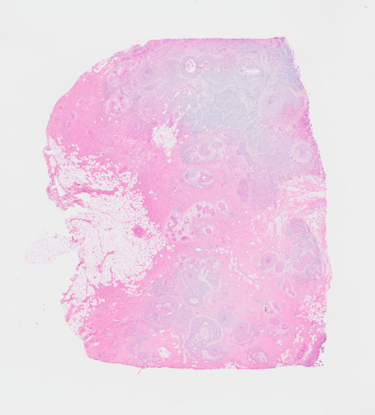
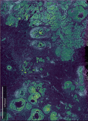
32 Workflow: Xenium + Visium

32.1 Preamble

32.1.1 Dependencies

Code

library(RANN)
library(scater)
library(scuttle)
library(harmony)
library(ggspavis)
library(VisiumIO)
library(patchwork)
library(OSTA.data)
library(BayesSpace)
library(SpatialExperiment)
library(SpatialExperimentIO)
# set seed for random number generation
# in order to make results reproducible
set.seed(194849)

32.1.2 Introduction

In this demo, we will rely on a dataset from Janesick et al. (2023), which includes same-section Visium and Xenium measurements on human breast cancer tissue.

H&E staining Xenium IF

32.2 Setup

We start out by retrieving these datasets from the OSF repository, and reading them into R as separate SpatialExperiment objects:

Code

# Visium
id <- "Visium_HumanBreast_Janesick"
pa <- OSTA.data_load(id)
dir.create(td <- tempfile())
unzip(pa, exdir=td)
obj <- TENxVisium(
    spacerangerOut=td, 
    images="lowres", 
    format="h5")
(vis <- import(obj))

##  class: SpatialExperiment 
##  dim: 18085 4992 
##  metadata(2): resources spatialList
##  assays(1): counts
##  rownames(18085): ENSG00000187634 ENSG00000188976 ... ENSG00000198695
##    ENSG00000198727
##  rowData names(3): ID Symbol Type
##  colnames(4992): AACACCTACTATCGAA-1 AACACGTGCATCGCAC-1 ...
##    TGTTGGCCAGACCTAC-1 TGTTGGCCTACACGTG-1
##  colData names(4): in_tissue array_row array_col sample_id
##  reducedDimNames(0):
##  mainExpName: Gene Expression
##  altExpNames(0):
##  spatialCoords names(2) : pxl_col_in_fullres pxl_row_in_fullres
##  imgData names(4): sample_id image_id data scaleFactor

Code

# Xenium
id <- "Xenium_HumanBreast1_Janesick"
pa <- OSTA.data_load(id)
dir.create(td <- tempfile())
unzip(pa, exdir=td)
(xen <- readXeniumSXE(td))

##  class: SpatialExperiment 
##  dim: 313 167780 
##  metadata(4): experiment.xenium transcripts cell_boundaries
##    nucleus_boundaries
##  assays(1): counts
##  rownames(313): ABCC11 ACTA2 ... ZEB2 ZNF562
##  rowData names(3): ID Symbol Type
##  colnames(167780): 1 2 ... 167779 167780
##  colData names(8): cell_id transcript_counts ... nucleus_area
##    sample_id
##  reducedDimNames(0):
##  mainExpName: NULL
##  altExpNames(4): NegControlProbe NegControlCodeword antisense BLANK
##  spatialCoords names(2) : x_centroid y_centroid
##  imgData names(0):

Code

# also retrieve cell subpopulation labels
df <- read.csv(file.path(td, "annotation.csv"))
xen$anno <- df$Annotation[match(xen$cell_id, df$Barcode)]

We’ll also do some data wrangling to simplify spatial coordinate names, and use gene symbols (rather than ensembl identifiers) as feature names for both data:

Code

# simplify spatial coordinate names
spatialCoordsNames(vis) <- spatialCoordsNames(xen) <- c("x", "y")
# use gene symbols as feature names
rownames(vis) <- make.unique(rowData(vis)$Symbol)
rownames(xen) <- make.unique(rowData(xen)$Symbol)

32.3 Alignment

To align Xenium and Visium sections, we use the affine transformation matrix provided by 10x Genomics, which was obtained by registration of Xenium onto Visium in Python with the Fiji (10xGenomics 2023) Java plug-in.

An affine map is generally composed of a linear map (scaling and rotation) and a translation, and can be apply using basic matrix multiplication and vector addition, specifically:

\[\mathbf{y}=A\mathbf{x}+\mathbf{b}\]

where \(A\) denotes the linear map, \(b\) the translation, and \(\mathbf{x}\) and \(\mathbf{y}\) correspond to original and transformed coordinates, respectively.

In R, this translates to the following operations:

Code

# affine matrix for aligning Xenium onto Visium
mtx <- matrix(nrow=2, byrow=TRUE, c(
    8.82797498e-02, -1.91831377e+00, 1.63476055e+04,
    1.84141210e+00,  5.96797885e-02, 4.12499099e+03),
    dimnames=list(c("x", "y"), c("x", "y", "z")))

Code

# stash original coordinates
old <- spatialCoords(xen)
colData(xen)[c(".x", ".y")] <- old
# apply affine transformation
new <- old %*% t(mtx[, -3]) # scale/rotate &
new <- sweep(new, 2, mtx[, 3], `+`) # offset
spatialCoords(xen) <- new

Code

df <- data.frame(spatialCoords(vis))
fd <- data.frame(spatialCoords(xen))
ggplot() + coord_equal() + theme_void() +
    geom_point(aes(x, y), df, col="grey", stroke=0, size=1) +
    geom_point(aes(x, y), fd, col="blue", stroke=0, size=0.1)

32.4 Aggregation

Binning single-cell resolution spatial data into spots can be useful for checking correlations between technical replicates of the same technology, identifying artifacts across technologies, and checking cell density (number of cells per spot). In general, it is possible to bin at the transcript-level (sub-cellular) or cell-level.

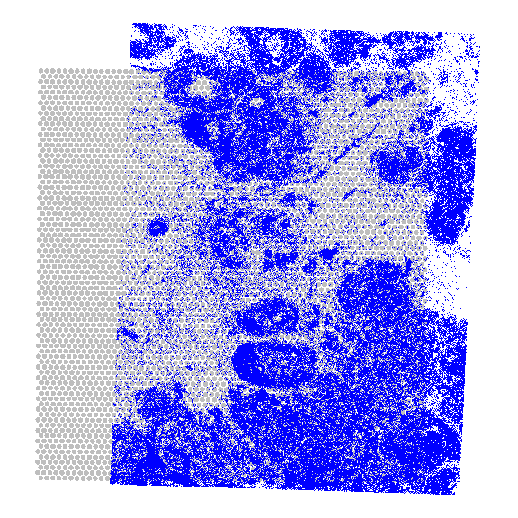
To aggregate single cell-level data from Xenium at the spot level, we first carry out a fixed-radius neighborhood search using RANN (c.f. Chapter 19) to identify, for ever spot, cells whose centroid lies within a \(\sim130\)um distance (Visium spot diameter of 55um, divided by two 2, divided by 0.2115 = Xenium px size in um):

Code

# do a fixed-radius search to get cell 
# centroids that fall on a given spot
nns <- nn2(
    searchtype="radius", radius=55/2/0.2125, k=200,
    data=spatialCoords(xen), query=spatialCoords(vis))

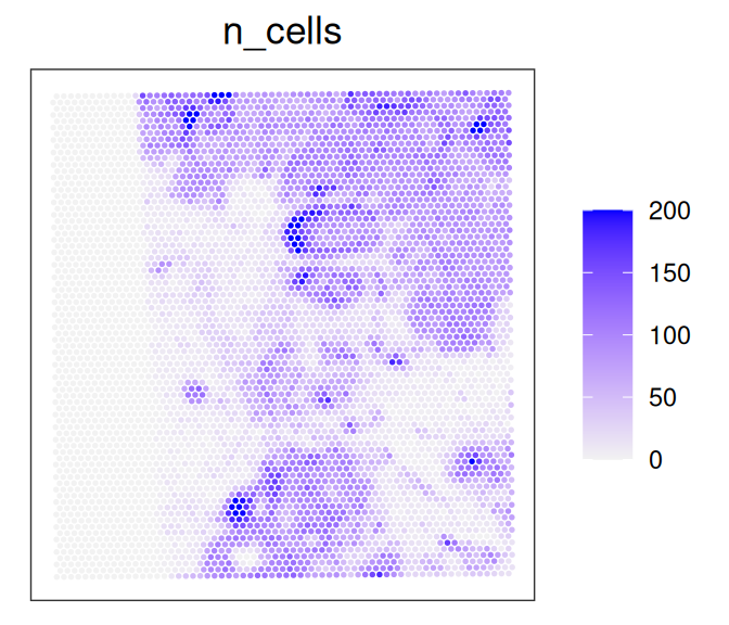
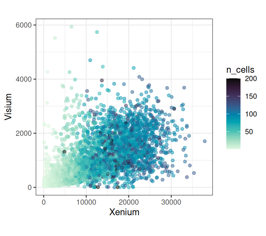
Let’s count and visualize the number of cells that overlap each spot:

Code

# get cell indices and number of cells per spot
vis$n_cells <- rowSums((idx <- nns$nn.idx) > 0)
plotSpots(vis, annotate="n_cells")

Next, we can aggregate single cell-level Xenium data into pseudo-spots. In addition, we propagate the Visium data’s spatial coordinates, excluding spots without any overlapping cells:

Code

# aggregate Xenium data into pseudo-spots
xem <- aggregateAcrossCells(xen[, c(t(idx))], rep.int(seq(ncol(vis)), vis$n_cells))
# propagate Visium data's spatial coordinates, excluding empty pseudo-spots
spatialCoords(xem) <- spatialCoords(vis)[vis$n_cells > 0, ] 
colnames(xem) <- colnames(vis)[vis$n_cells > 0]
xem$in_tissue <- 1

Because we’ve aligned the Xenium to the Visium data, we can also propagate the Visium data’s imgData (low resolution H&E staining) to the object containing pseudo-spot Xenium data:

Code

imgData(xem) <- imgData(vis)

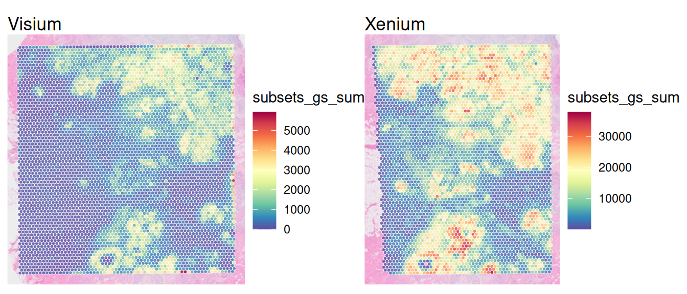
Next, let’s compute some standard quality control metrics on both, the Visium and pseudo-spot Xenium data. Besides dataset-specific metrics, we also specify the subset of genes that are shared between both datasets in order to obtain comparable metrics:

Code

sub <- list(gs=intersect(rownames(vis), rownames(xen)))
vis <- addPerCellQCMetrics(vis, subsets=sub)
xem <- addPerCellQCMetrics(xem, subsets=sub)

Let’s visually compare the total counts per (pseudo-)spot between Visium and Xenium:

Code

plotVisium(vis, 
    annotate="subsets_gs_sum",
    zoom=TRUE, facets=NULL) +
    ggtitle("Visium") +
plotVisium(xem, 
    annotate="subsets_gs_sum",
    zoom=TRUE, facets=NULL) +
    ggtitle("Xenium") +
plot_layout(nrow=1)

We can also use a scatter plot - where points = (pseudo-)spots - to directly compare total counts between both technologies:

Code

df <- data.frame(
    n_cells=xem$ncells,
    Xenium=xem$subsets_gs_sum,
    Visium=vis[, colnames(xem)]$subsets_gs_sum)
ggplot(df, aes(Xenium, Visium, col=n_cells)) + 
    scale_color_gradientn(colors=rev(hcl.colors(9, "Mako"))) +
    geom_point(alpha=0.5) + theme_bw() + theme(aspect.ratio=1)

32.5 Integration

Besides physically aligning both datasets, we can integrate them on a transcriptional level; here, using harmony.

To this end, we first consolidate the Visium and Xenium data into one object:

Code

# pool datasets together
gs <- intersect(rownames(vis), rownames(xem))
cs <- intersect(colnames(vis), colnames(xem))
cd <- intersect(names(colData(vis)), names(colData(xem)))
lys <- list(Visium=vis, Xenium=xem)
lys <- mapply(spe=lys, sid=names(lys), \(spe, sid) {
    spe <- spe[gs, cs]
    spe$sample_id <- sid
    rowData(spe) <- NULL
    colData(spe) <- colData(spe)[cd]
    assay(spe) <- as(assay(spe), "dgCMatrix")
    return(spe)
}, SIMPLIFY=FALSE)
(obj <- do.call(cbind, lys))

##  class: SpatialExperiment 
##  dim: 307 7954 
##  metadata(6): resources spatialList ... cell_boundaries
##    nucleus_boundaries
##  assays(1): counts
##  rownames(307): FBLIM1 C1QA ... IL2RG TCEAL7
##  rowData names(0):
##  colnames(7954): AACACGTGCATCGCAC-1 AACACTTGGCAAGGAA-1 ...
##    TGTTGGATGGACTTCT-1 TGTTGGCCAGACCTAC-1
##  colData names(8): in_tissue sample_id ... subsets_gs_percent total
##  reducedDimNames(0):
##  mainExpName: Gene Expression
##  altExpNames(0):
##  spatialCoords names(2) : x y
##  imgData names(4): sample_id image_id data scaleFactor

In order to perform joint spatial clustering of both modalities, we construct array coordinates for Xenium pseudo-spots that are offset from Visium spots:

Code

# offset the spatial location for joint clustering
# of Visium and adjacent pseudo-spot Xenium data
obj$array_row <- c(ar <- vis[, cs]$array_row, 100+ar)
obj$array_col <- c(ac <- vis[, cs]$array_col, 100+ac)

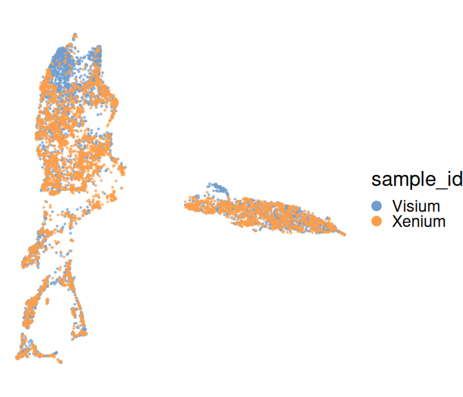
Next, we run a standard pipeline to perform log-library size normalization (using scater), principal component analysis (PCA), harmony integration, and dimension reduction (UMAP). Notably, the feature selection step that typically precedes PCA is skipped here, as the Xenium experiment includes only a curated selection of \(\sim300\) targets by design.

Code

# minimal filtering
obj <- obj[, obj$subsets_gs_sum > 0]
# library size normalization 
obj <- logNormCounts(obj)
# principal component analysis
# (w/o additional feature selection)
obj <- runPCA(obj)
# 'harmony' integration
pcs <- RunHarmony(
    data_mat=reducedDim(obj, "PCA"), 
    meta_data=obj$sample_id, 
    verbose=FALSE)
reducedDim(obj, "PCA") <- pcs
# dimensionality reduction
map <- calculateUMAP(t(pcs))
reducedDim(obj, "UMAP") <- map

Code

plotUMAP(obj, colour_by="sample_id", point_size=0.1) +
    guides(col=guide_legend(override.aes=list(alpha=1, size=2))) +
    theme_void() + theme(aspect.ratio=1, legend.key.size=unit(0, "pt"))

32.6 Clustering

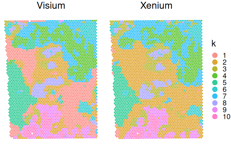
The spatialCluster() function clusters the spots, and adds the predicted cluster labels to the object. The authors recommend running with at least 10,000 iterations (nrep=1e4); we use fewer iterations in this demo for the sake of runtime. (Note that a random seed must be set (set.seed()) for the results to be reproducible.)

Code

# 'BayesSpace' clustering
res <- spatialCluster(obj, q=10, burn.in=100, nrep=1e3)
table(res$k <- factor(res$spatial.cluster))

##  
##     1    2    3    4    5    6    7    8    9   10 
##   877 1958  642 1042  796  396 1033  435  497  277

We see high concordance between the two modalities, although the aggregated Xenium data appears to yield slightly higher granularity:

Code

plotVisium(res, 
    image=FALSE, annotate="k") +
    theme(legend.key.size=unit(0, "pt"))

From here on out, both datasets could be analyzed together and/or independently, e.g., in order to identify cluster markers, annotate cell subpopulations etc.

32.7 Appendix

References

10xGenomics. 2023. H&e to Xenium DAPI Image Registration with Fiji. https://www.10xgenomics.com/resources/analysis-guides/he-to-xenium-dapi-image-registration-with-fiji#.

Janesick, Amanda, Robert Shelansky, Andrew D. Gottscho, Florian Wagner, Stephen R. Williams, Morgane Rouault, Ghezal Beliakoff, et al. 2023. “High Resolution Mapping of the Tumor Microenvironment Using Integrated Single-Cell, Spatial and in Situ Analysis.” Nature Communications 14 (1): 8353.