29 Differential spatial patterns

29.1 Preamble

29.1.1 Introduction

Recent advances in spatial transcriptomics (ST) techniques have facilitated the generation of multi-sample datasets across various experimental conditions (e.g. healthy vs. diseased, or multiple treatments).

When multi-sample, multi-condition ST data are available, differential analysis can be performed to identify genes with distinct spatial expression patterns between conditions, which we call differential spatial pattern (DSP) genes. A DSP gene may be spatially variable in one condition and display spatially uniform expression in another one, or it could be spatially variable in all conditions, but with distinct spatial expression patterns. Conversely, genes that show spatially uniform abundance, or that are spatially variable with the same spatial structure in all conditions, are not considered DSP, because their spatial distribution is unchanged.

Identifying DSP genes can provide valuable insights into how gene expression spatial structures change across experimental conditions, helping to understand the underlying biological processes.

29.1.2 Dependencies

Code

library(muSpaData)
library(ggspavis)
library(DESpace)
library(edgeR)

29.1.3 Load data

In this demo, we will analyze a Stereo-seq dataset from axolotl brain tissues collected at various stages of regeneration (Wei et al. 2022), which includes multiple samples (i.e. serial sections) measured under multiple experimental conditions (regeneration stages).

In the original dataset, which is publicly available through the Spatial Transcript Omics DataBase, there are 5 stages with multiple sections, totaling 16 samples (3 to 4 sections per stage).

In this chapter, for computational reasons, we use 3 stages – 2, 10, and 20 days post injury (DPI) – and only two sections per stage. The analysis framework uses pre-computed spatial domains generated with Banksy (Singhal et al. 2024). For performing clustering with Banksy, refer to Chapter 22. For preprocessing details of this dataset, see the muSpaData Bioconductor package.

Code

spe <- Wei22_example()

Code

colnames(spatialCoords(spe)) <- c("x", "y")
plotCoords(spe, 
    annotate = "Banksy_smooth", 
    in_tissue = NULL, 
    x_coord = "sdimx", 
    y_coord = "sdimy", 
    sample_id = "sample_id") + 
    theme(legend.key.size = unit(0, "lines")) + 
    scale_color_manual(values=unname(pals::trubetskoy()))

29.2 DESpace

Here, we briefly demonstrate how to identify DSP genes using the DESpace (Cai, Robinson, and Tiberi 2024) Bioconductor package. For more details see the package vignette.

Code

# run DESpace
dsp <- dsp_test(spe = spe, cluster_col = "Banksy_smooth", 
                sample_col = "sample_id", condition_col = "condition", 
                verbose = TRUE)

Code

head(dsp_global <- dsp$gene_results, n = 3)

##                        gene_id logFC.condition20DPI.cluster_id1
##  AMEX60DD014721 AMEX60DD014721                      -0.07170723
##  AMEX60DD045083 AMEX60DD045083                       0.08759059
##  AMEX60DD011151 AMEX60DD011151                      -0.97377297
##                 logFC.condition2DPI.cluster_id1
##  AMEX60DD014721                      -0.3898784
##  AMEX60DD045083                       0.5418637
##  AMEX60DD011151                      -2.1019048
##                 logFC.condition20DPI.cluster_id2
##  AMEX60DD014721                       -0.8510223
##  AMEX60DD045083                       -1.3377605
##  AMEX60DD011151                        0.1861520
##                 logFC.condition2DPI.cluster_id2
##  AMEX60DD014721                       0.8526301
##  AMEX60DD045083                       1.1226997
##  AMEX60DD011151                       0.4671347
##                 logFC.condition20DPI.cluster_id3
##  AMEX60DD014721                       -0.8328237
##  AMEX60DD045083                        0.2478193
##  AMEX60DD011151                       -0.4011555
##                 logFC.condition2DPI.cluster_id3
##  AMEX60DD014721                      -0.9450830
##  AMEX60DD045083                       1.2666344
##  AMEX60DD011151                       0.4086612
##                 logFC.condition20DPI.cluster_id4
##  AMEX60DD014721                       0.22287797
##  AMEX60DD045083                      -0.99648014
##  AMEX60DD011151                      -0.01634095
##                 logFC.condition2DPI.cluster_id4   logCPM        LR
##  AMEX60DD014721                       0.2085777 9.344907 100.69288
##  AMEX60DD045083                      -0.7969334 7.505402  97.72697
##  AMEX60DD011151                       0.1810959 7.959492  85.69149
##                       PValue          FDR
##  AMEX60DD014721 3.081052e-18 1.540526e-14
##  AMEX60DD045083 1.243325e-17 3.108313e-14
##  AMEX60DD011151 3.472538e-15 5.787563e-12

Code

# count significant DSP genes (at 5% FDR significance level)
table(dsp_global$FDR <= 0.05)

##  
##  FALSE  TRUE 
##   4809   191

In order to identify the key spatial cluster where expression changes across conditions, we use individual_dsp() function.

Code

dsp_clu <- individual_dsp(spe, cluster_col = "Banksy_smooth", 
                          sample_col = "sample_id", condition_col = "condition")

Code

# results for cluster 2
dsp_clu2 <- dsp_clu$`2`
head(dsp_clu2, n = 3)

##                        gene_id logFC.condition20DPI.cluster_id2
##  AMEX60DD014721 AMEX60DD014721                       -0.5801351
##  AMEX60DD014991 AMEX60DD014991                        2.6944195
##  AMEX60DD055246 AMEX60DD055246                       -0.2660938
##                 logFC.condition2DPI.cluster_id2   logCPM       LR
##  AMEX60DD014721                        1.270051 9.582333 74.62550
##  AMEX60DD014991                        3.015258 7.330327 73.65886
##  AMEX60DD055246                       -2.298605 5.661946 61.49402
##                       PValue          FDR
##  AMEX60DD014721 6.241352e-17 2.530002e-13
##  AMEX60DD014991 1.012001e-16 2.530002e-13
##  AMEX60DD055246 4.433456e-14 7.389093e-11

Code

# top DSP gene for cluster 2
top_dsp <- dsp_clu2$gene_id[1]

# get gene symbols from Ensembl identifiers
idx <- match(top_dsp, rowData(spe)$gene_name)
(.gs <- rowData(spe)$gene_id[idx])

##  [1] "ECM1"

29.3 Visualization

DSP genes can be further investigated, for example, by plotting the spatial expression of genes across groups, or the log2-transformed counts per million of genes across different clusters and groups.

Code

plotCoords(spe, 
    annotate = .gs, 
    assay_name = "logcounts", 
    feature_names = "gene_id", 
    in_tissue = NULL, 
    x_coord = "sdimx", 
    y_coord = "sdimy", 
    sample_id = "sample_id") + 
    theme(legend.key.size=unit(1, "lines"))

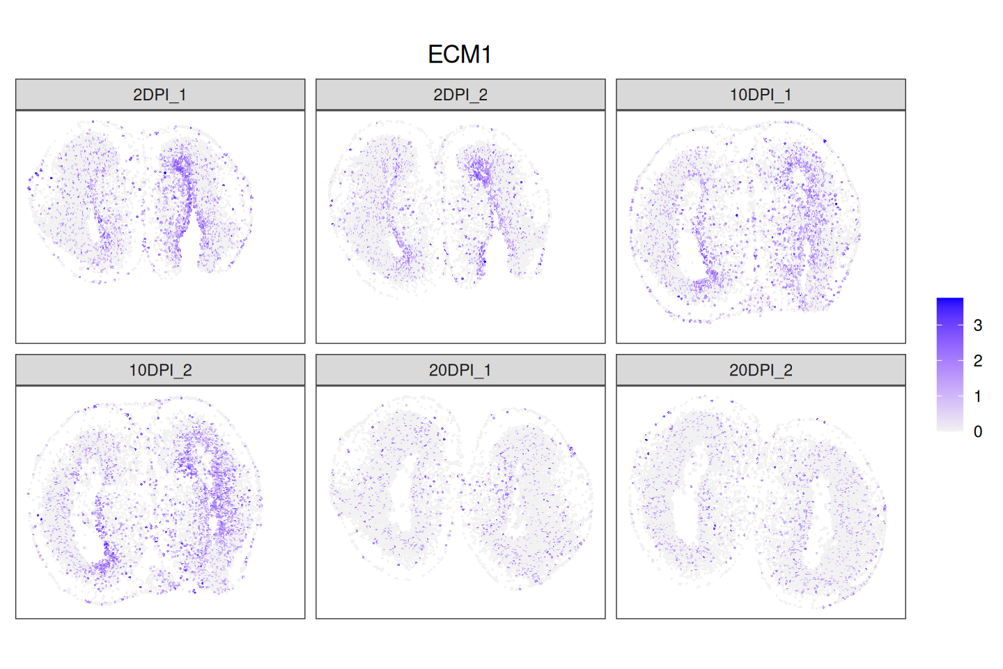
Code

# calculate log CPM
cps <- edgeR::cpm(dsp$estimated_y, log = TRUE)
cps_name <- colnames(cps)
mdata <- data.frame(
    log_cpm = cps[top_dsp, ], 
    Banksy_smooth = factor(sub(".*_", "", cps_name)), 
    day = as.numeric(sub("([0-9]+)DPI.*", "\\1", cps_name)), 
    sample_id = sub("(_[0-9]+)$", "", cps_name)
)

ggplot(mdata, aes(x = factor(day), y = log_cpm)) + 
    geom_jitter(aes(color = Banksy_smooth), size = 2, width = 0.1) + 
    geom_boxplot(aes(fill = ifelse(Banksy_smooth == "2", 
                                   "cluster 2", "non-cluster 2"))) + 
    scale_x_discrete(breaks = c(2, 10, 20)) + 
    scale_fill_manual(values = c("#4DAF4A", "gray")) + 
    labs(title = .gs, x = "Days post injury", 
         y = "log2 counts per million (logCPM)", fill = "", 
         color = "Banksy cluster") + 
     theme(legend.position = "right")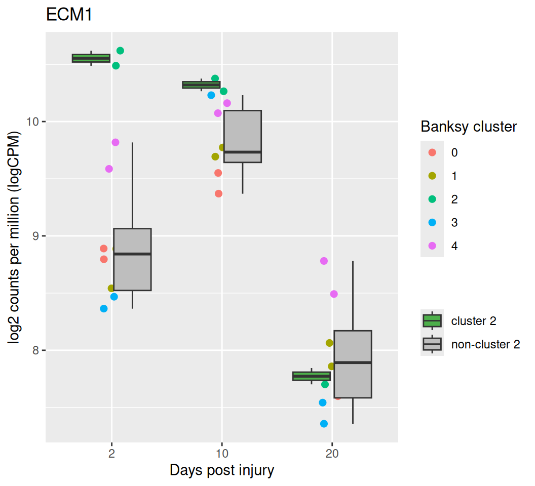

The boxplots above show the average log-CPM for cluster 2 and for all other clusters (excluding cluster 2) across different time phases. The largest difference between cluster 2 and the remaining clusters is observed at 2 DPI, with the difference decreasing over time. At 20 DPI, no significant log-CPM differences are observed between the clusters. This suggests that spatial patterns change across conditions (i.e. time stages).

29.4 Appendix

References

Cai, Peiying, Mark D Robinson, and Simone Tiberi. 2024. “DESpace: Spatially Variable Gene Detection via Differential Expression Testing of Spatial Clusters.” Bioinformatics 40 (2): btae027.

Singhal, Vipul, Nigel Chou, Joseph Lee, Yifei Yue, Jinyue Liu, Wan Kee Chock, Li Lin, et al. 2024. “BANKSY Unifies Cell Typing and Tissue Domain Segmentation for Scalable Spatial Omics Data Analysis.” Nature Genetics 56 (3): 431–41.

Wei, Xiaoyu, Sulei Fu, Hanbo Li, Yang Liu, Shuai Wang, Weimin Feng, Yunzhi Yang, et al. 2022. “Single-Cell Stereo-Seq Reveals Induced Progenitor Cells Involved in Axolotl Brain Regeneration.” Science 377: 1062. https://doi.org/10.1126/science.abp9444.