11 Workflow: Visium DLPFC

11.1 Preamble

11.1.1 Introduction

This workflow analyzes a 10x Genomics Visium dataset consisting of one sample (Visium capture area) of postmortem human brain tissue from the dorsolateral prefrontal cortex (DLPFC) region, originally described by Maynard et al. (2021).

The original full dataset contains 12 samples in total, from 3 donors, with 2 pairs of spatially adjacent replicates (serial sections) per donor (4 samples per donor). Each sample spans several cortical layers plus white matter in a tissue section. The examples in this workflow use a single representative sample (sample 151673).

For more details on the dataset, see Maynard et al. (2021). The full dataset is publicly available through the spatialLIBD Bioconductor package (Pardo et al. 2022). The dataset can also be explored interactively through the spatialLIBD Shiny web app.

11.1.2 Dependencies

Code

library(SpatialExperiment)
library(STexampleData)
library(ggspavis)
library(patchwork)
library(scater)
library(scran)
library(pheatmap)

11.2 Workflow

11.2.1 Load data

Load sample 151673 from the DLPFC dataset. This sample is available as a SpatialExperiment object from the STexampleData package.

Code

# load data
spe <- Visium_humanDLPFC()

class(spe)

##  [1] "SpatialExperiment"
##  attr(,"package")
##  [1] "SpatialExperiment"

Code

dim(spe)

##  [1] 33538  4992

11.2.2 Plot data

As an initial check, plot the spatial coordinates (spots) in x-y dimensions, to check that the object has loaded correctly. We use plotting functions from the ggspavis package.

Code

# plot spatial coordinates (spots)
plotCoords(spe)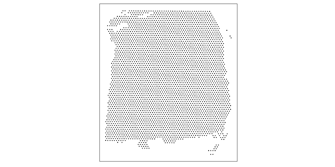

11.2.3 Quality control (QC)

We calculate quality control (QC) metrics using the scater package (McCarthy et al. 2017), and apply simple global thresholding-based QC methods to identify any low-quality spots, as described in Section 8.3.

For more details on QC methods, including more advanced QC approaches, see Chapter 8.

Code

# subset to keep only spots over tissue
spe <- spe[, colData(spe)$in_tissue == 1]
dim(spe)

##  [1] 33538  3639

Code

# identify mitochondrial genes
is_mito <- grepl("(^MT-)|(^mt-)", rowData(spe)$gene_name)
table(is_mito)

##  is_mito
##  FALSE  TRUE 
##  33525    13

Code

rowData(spe)$gene_name[is_mito]

##   [1] "MT-ND1"  "MT-ND2"  "MT-CO1"  "MT-CO2"  "MT-ATP8" "MT-ATP6" "MT-CO3" 
##   [8] "MT-ND3"  "MT-ND4L" "MT-ND4"  "MT-ND5"  "MT-ND6"  "MT-CYB"

Calculate QC metrics using scater (McCarthy et al. 2017).

Code

# calculate per-spot QC metrics and store in colData
spe <- addPerCellQC(spe, subsets = list(mito = is_mito))
head(colData(spe), 3)

##  DataFrame with 3 rows and 14 columns
##                             barcode_id     sample_id in_tissue array_row
##                            <character>   <character> <integer> <integer>
##  AAACAAGTATCTCCCA-1 AAACAAGTATCTCCCA-1 sample_151673         1        50
##  AAACAATCTACTAGCA-1 AAACAATCTACTAGCA-1 sample_151673         1         3
##  AAACACCAATAACTGC-1 AAACACCAATAACTGC-1 sample_151673         1        59
##                     array_col ground_truth   reference cell_count       sum
##                     <integer>  <character> <character>  <integer> <numeric>
##  AAACAAGTATCTCCCA-1       102       Layer3      Layer3          6      8458
##  AAACAATCTACTAGCA-1        43       Layer1      Layer1         16      1667
##  AAACACCAATAACTGC-1        19           WM          WM          5      3769
##                      detected subsets_mito_sum subsets_mito_detected
##                     <integer>        <numeric>             <integer>
##  AAACAAGTATCTCCCA-1      3586             1407                    13
##  AAACAATCTACTAGCA-1      1150              204                    11
##  AAACACCAATAACTGC-1      1960              430                    13
##                     subsets_mito_percent     total
##                                <numeric> <numeric>
##  AAACAAGTATCTCCCA-1              16.6351      8458
##  AAACAATCTACTAGCA-1              12.2376      1667
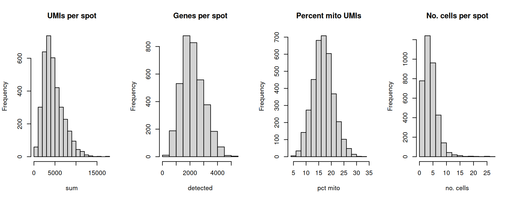
##  AAACACCAATAACTGC-1              11.4089      3769

Select global filtering thresholds for the QC metrics by examining distributions using histograms.

Code

par(mfrow = c(1, 4))
hist(spe$sum, xlab = "sum", main = "UMIs per spot")
hist(spe$detected, xlab = "detected", main = "Genes per spot")
hist(spe$subsets_mito_percent, xlab = "pct mito", main = "Percent mito UMIs")
hist(spe$cell_count, xlab = "no. cells", main = "No. cells per spot")

Code

par(mfrow = c(1, 1))

Code

# select global QC thresholds
spe$qc_lib_size <- spe$sum < 600
spe$qc_detected <- spe$detected < 400
spe$qc_mito <- spe$subsets_mito_percent > 28

table(spe$qc_lib_size)

##  
##  FALSE  TRUE 
##   3631     8

Code

table(spe$qc_detected)

##  
##  FALSE  TRUE 
##   3632     7

Code

table(spe$qc_mito)

##  
##  FALSE  TRUE 
##   3622    17

Plot the spatial distributions of the potentially identified low-quality spots, to ensure that they are not concentrated within biologically meaningful regions (which could suggest that the selected thresholds were too stringent).

Code

# plot spatial distributions of discarded spots
p1 <- plotObsQC(spe, plot_type = "spot", annotate = "qc_lib_size") + 
  ggtitle("Library size (< threshold)")
p2 <- plotObsQC(spe, plot_type = "spot", annotate = "qc_detected") + 
  ggtitle("Detected genes (< threshold)")
p3 <- plotObsQC(spe, plot_type = "spot", annotate = "qc_mito") + 
  ggtitle("Mito proportion (> threshold)")

# arrange plots using patchwork package
p1 | p2 | p3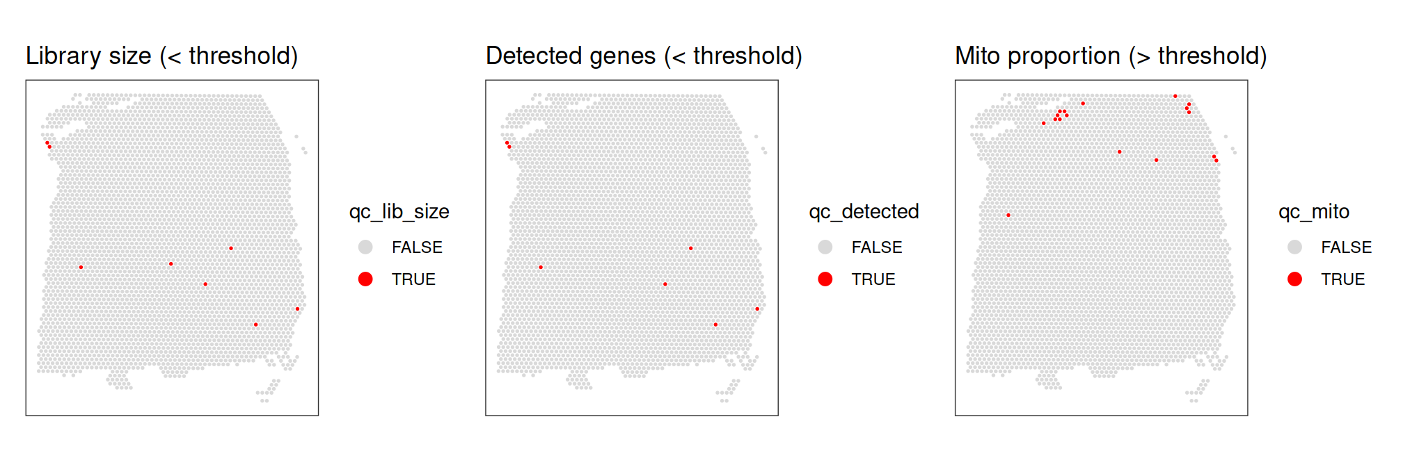

Select spots to discard by combining the sets of identified low-quality spots according to each metric.

Code

# number of identifed spots for each metric
apply(cbind(spe$qc_lib_size, spe$qc_detected, spe$qc_mito), 2, sum)

##  [1]  8  7 17

Code

# combined set of identified spots
spe$discard <- spe$qc_lib_size | spe$qc_detected | spe$qc_mito
table(spe$discard)

##  
##  FALSE  TRUE 
##   3614    25

Plot the spatial distribution of the combined set of identified low-quality spots to discard, to again confirm that they do not correspond to any clearly biologically meaningful regions, which could indicate that we are removing biologically informative spots. Specifically, in this dataset, we want to ensure that the discarded spots do not correspond to a single cortical layer.

Code

# check spatial pattern of discarded spots
plotObsQC(spe, plot_type = "spot", annotate = "discard")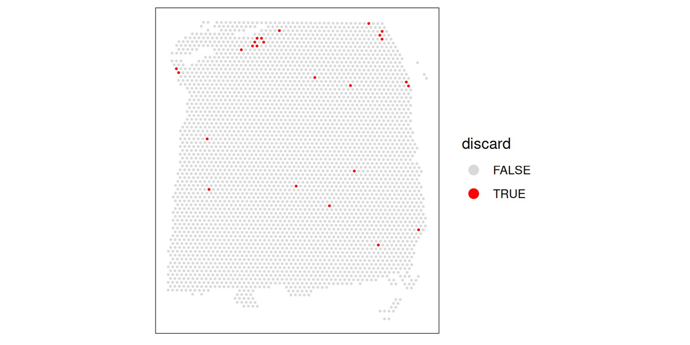

Filter out the low-quality spots.

Code

# filter out low-quality spots
spe <- spe[, !spe$discard]
dim(spe)

##  [1] 33538  3614

11.2.4 Normalization

Calculate log-transformed normalized counts (logcounts) using library size normalization, as described in Section 9.2. We use methods from the scater (McCarthy et al. 2017) and scran (Lun, McCarthy, and Marioni 2016) packages, making the simplified assumption that spots can be treated as equivalent to single cells. For more details, see Chapter 9.

Code

# calculate library size factors
spe <- computeLibraryFactors(spe)

summary(sizeFactors(spe))

##     Min. 1st Qu.  Median    Mean 3rd Qu.    Max. 
##   0.1330  0.6329  0.8978  1.0000  1.2872  3.7820

Code

hist(sizeFactors(spe), breaks = 20, main = "Histogram of size factors")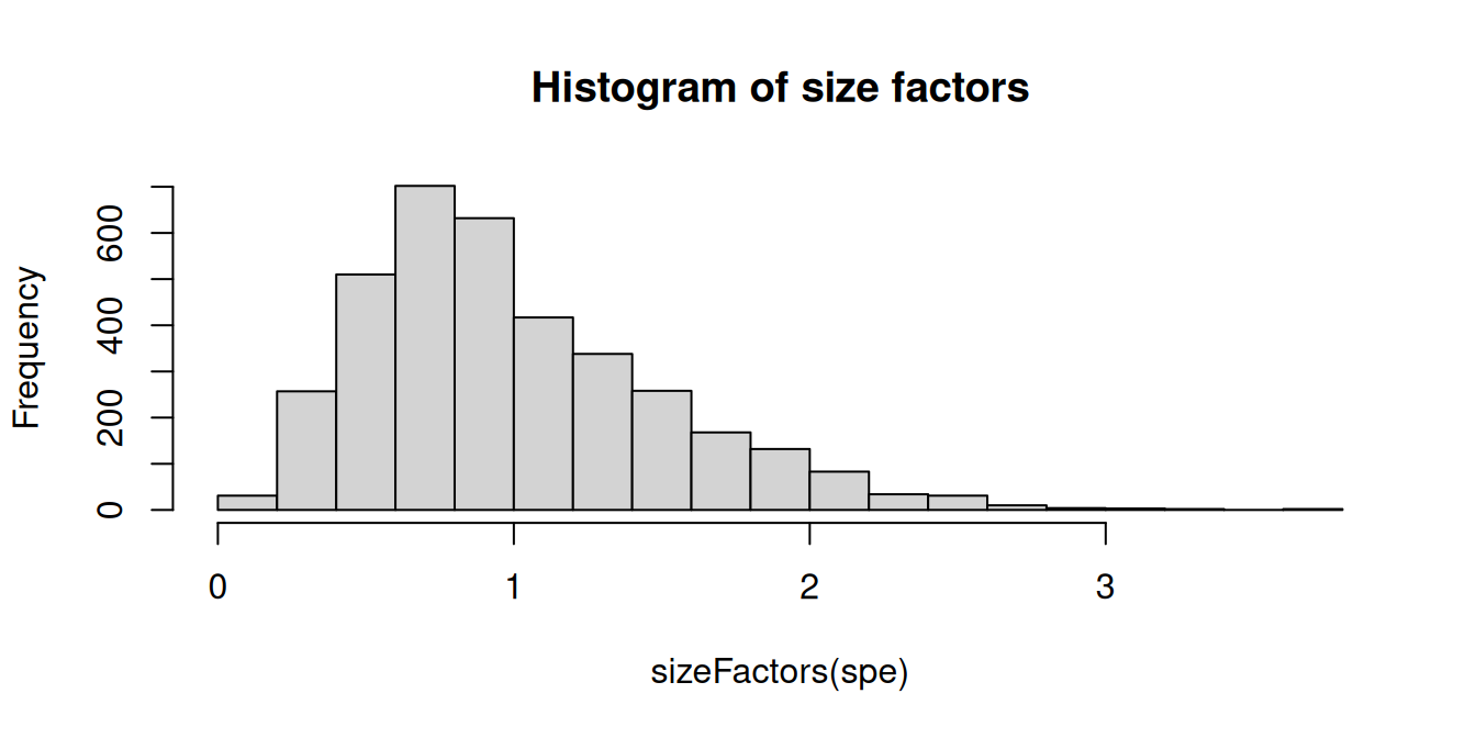

Code

# calculate logcounts
spe <- logNormCounts(spe)

assayNames(spe)

##  [1] "counts"    "logcounts"

11.2.5 Feature selection (HVGs)

Apply feature selection methods to identify a set of top highly variable genes (HVGs). We use methods from the scran (Lun, McCarthy, and Marioni 2016) package, again making the simplified assumption that spots can be treated as equivalent to single cells. We also first remove mitochondrial genes, since these tend to be very highly expressed and are not of main biological interest.

For more details, see Chapter 9.

For details on alternative feature selection methods to identify spatially variable genes (SVGs) instead of HVGs, for example using the nnSVG (Weber et al. 2023) or other packages, see Chapter 23.

Code

# remove mitochondrial genes
spe <- spe[!is_mito, ]
dim(spe)

##  [1] 33525  3614

Code

# fit mean-variance relationship, decomposing variance into 
# technical and biological components
dec <- modelGeneVar(spe)

# select top HVGs
top_hvgs <- getTopHVGs(dec, prop = 0.1)

# number of HVGs selected
length(top_hvgs)

##  [1] 1424

11.2.6 Dimensionality reduction

Next, we perform dimensionality reduction using principal component analysis (PCA), applied to the set of top HVGs. We retain the top 50 principal components (PCs) for further downstream analyses. This is done both to reduce noise and to improve computational efficiency. We also run UMAP on the set of top 50 PCs and retain the top 2 UMAP components for visualization purposes.

We use the computationally efficient implementation of PCA from the scater package (McCarthy et al. 2017), which uses randomization and therefore requires setting a random seed for reproducibility.

See Chapter 9 and Chapter 21 for more details.

Code

# using scater package
set.seed(123)
spe <- runPCA(spe, subset_row = top_hvgs)
spe <- runUMAP(spe, dimred = "PCA")

reducedDimNames(spe)

##  [1] "PCA"  "UMAP"

Code

dim(reducedDim(spe, "PCA"))

##  [1] 3614   50

Code

dim(reducedDim(spe, "UMAP"))

##  [1] 3614    2

Code

# update column names for plotting
colnames(reducedDim(spe, "UMAP")) <- paste0("UMAP", 1:2)

11.2.7 Clustering

Next, we apply a clustering algorithm to identify cell types or spatial domains. Note that we are using only molecular features (gene expression) as the input for clustering in this example. Alternatively, we could use a spatially-aware clustering algorithm, as demonstrated in the example in Section 9.5.

Here, we use graph-based clustering using the Walktrap method implemented in scran, applied to the top 50 PCs calculated on the set of top HVGs from above.

For more details on clustering, see Chapter 22.

Code

# graph-based clustering
set.seed(123)
k <- 10
g <- buildSNNGraph(spe, k = k, use.dimred = "PCA")
g_walk <- igraph::cluster_walktrap(g)
clus <- g_walk$membership
table(clus)

##  clus
##    1   2   3   4   5   6   7 
##  365 765 875 803 198 370 238

Code

# store cluster labels in column 'label' in colData
colLabels(spe) <- factor(clus)

Visualize the cluster labels by plotting in x-y space, alongside the manually annotated reference labels (ground_truth) available for this dataset.

Code

# plot cluster labels in x-y space
plotCoords(spe, annotate = "label", pal = "libd_layer_colors")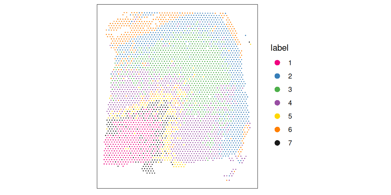

Code

# plot manually annotated reference labels
plotCoords(spe, annotate = "ground_truth", pal = "libd_layer_colors")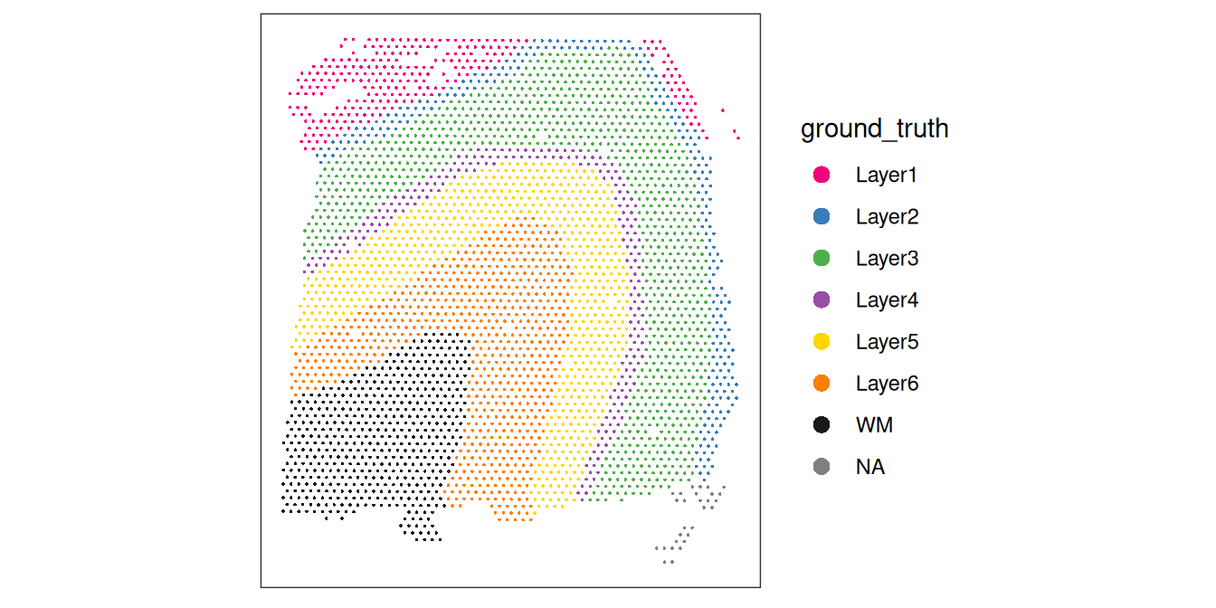

We can also plot the cluster labels in the top 2 UMAP dimensions.

Code

# plot clusters labels in UMAP dimensions
plotDimRed(spe, plot_type = "UMAP", annotate = "label", 
           pal = "libd_layer_colors")

11.2.8 Differential expression

Identify marker genes for each cluster or spatial domain by testing for differentially expressed genes using pairwise t-tests, specifically testing for upregulation for each cluster or spatial domain.

We use the scran package (Lun, McCarthy, and Marioni 2016) to calculate the differential tests. We use a binomial test, which is a more stringent test than the default pairwise t-tests, and tends to select genes that are easier to interpret and validate experimentally.

See Chapter 9 or Chapter 22 for more details.

Code

# using scran package
mgs <- findMarkers(spe, groups = spe$label, test = "binom", direction = "up")
top <- lapply(mgs, \(df) rownames(df)[df$Top <= 3])
length(top <- unique(unlist(top)))

##  [1] 67

Visualize the marker genes using a heatmap.

Code

pbs <- aggregateAcrossCells(spe, 
  ids = spe$label, subset.row = top, 
  use.assay.type = "logcounts", statistics = "mean")

# use gene symbols as feature names
mtx <- t(assay(pbs))
colnames(mtx) <- rowData(pbs)$gene_name

# plot using pheatmap package
pheatmap(mat = mtx, scale = "column")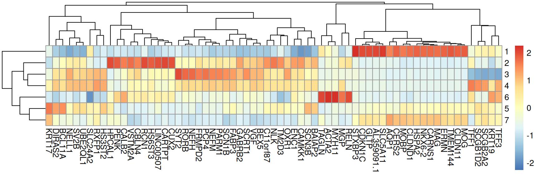

11.3 spatialLIBD

The examples above demonstrated a streamlined analysis workflow for the Visium DLPFC dataset (Maynard et al. 2021). In this section, we will use the spatialLIBD package (Pardo et al. 2022) to continue analyzing this dataset by creating an interactive Shiny website to visualize the data.

11.3.1 Why use spatialLIBD?

The spatialLIBD package has a function, spatialLIBD::run_app(spe), which will create an interactive website using a SpatialExperiment object (spe). The interactive website it creates has several features that were initially designed for the DLPFC dataset (Maynard et al. 2021) and later made flexible for any dataset (Pardo et al. 2022). These features include panels to visualize Visium spots:

for one tissue section at a time, either with interactive or static versions
for multiple tissue sections at a time, either interactively or statically

Both options work with continuous and discrete variables such as the gene expression and clusters, respectively. The interactive version for discrete variables such as clusters is useful if you want to manually annotate Visium spots, as in Maynard et al. (2021). spatialLIBD allows users to download the annotated spots and resume your spot annotation work later.

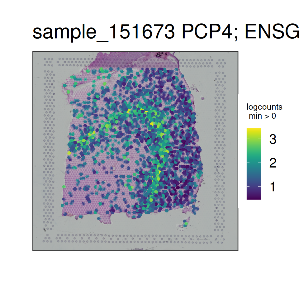
Screenshot of the ‘clusters (interactive)’ section of the ‘spot-level data’ panel created with the full spatialLIBD dataset. The website was created with `spatialLIBD::run_app(spatialLIBD::fetch_data('spe'))` version 1.4.0 and then using the lasso selection, we selected a set of spots in the UMAP interactive plot colored by the estimated number of cells per spot (`cell_count`) on the bottom left, which automatically updated the other three plots.

Visualizing genes or clusters across multiple tissue sections can be useful. For example, here we show the expression levels of PCP4 across two sets of spatially adjacent replicates. PCP4 is a marker gene for layer 5 in the gray matter of the DLPFC in the human brain. Spatially adjacent replicates are about 10 μm apart from each other and visualizations like the one below help assess the technical variability in the Visium technology.

Screenshot of the ‘gene grid (static)’ section of the ‘spot-level data’ panel created with the full spatialLIBD dataset. The website was created with `spatialLIBD::run_app(spatialLIBD::fetch_data('spe'))` version 1.4.0, selecting the *PCP4* gene, selecting the *paper* gene color scale, changing the number of rows and columns in the grid 2, selecting two pairs of spatially adjacent replicate samples (151507, 151508, 151673, and 151674), and clicking on the *upgrade grid plot* button. Note that the default *viridis* gene color scale is color-blind friendly.

You can try out a spatialLIBD-powered website yourself by opening it on your browser.

Check https://github.com/LieberInstitute/spatialLIBD#shiny-website-mirrors in case you need to use a mirror. shiny-powered websites work best on browsers such as Google Chrome and Mozilla Firefox, among others.

11.3.2 Want to learn more about spatialLIBD?

For more details about spatialLIBD, please check the spatialLIBD Bioconductor landing page or the pkgdown documentation website. In particular, we have two vignettes:

You can also read more about spatialLIBD in the associated publication Pardo et al. (2022).

If you prefer to watch videos, recorded presentations related to the dataset (Maynard et al. 2021) and spatialLIBD (Pardo et al. 2022) are also available here.

11.3.3 Code prerequisites

For this demo, we will re-use the spe object (in `r BiocStyle::Biocpkg(“SpatialExperiment”) format) created in the example DLPFC workflow above. If you are starting from here, you can re-build the object by running the code in section Section 11.2 above.

We also load some additional dependency packages, in addition to the dependencies already loaded in Section 11.2 above.

Code

library(BiocFileCache)  # for downloading and storing data
library(rtracklayer)  # for importing gene annotation files

##  
##  Attaching package: 'rtracklayer'

##  The following object is masked from 'package:AnnotationHub':
##  
##      hubUrl

In addition, we will modify the final step of the workflow above, where we identified marker genes per cluster by differential expression testing. We will modify this step to summarize the results of the differential expression testing in a different way, and store this information in the spe object.

Code

# identify interesting markers for each cluster
interesting <- sapply(mgs, function(x) x$Top <= 5)
colnames(interesting) <- paste0("gene_interest_", seq_len(length(mgs)))
rowData(spe) <- cbind(rowData(spe), interesting)

11.3.4 Prepare for spatialLIBD

We also need to modify the spe object, similar to steps we need to carry out when using spatialLIBD with 10x Genomics public datasets.

11.3.4.1 Basic information

Code

# add some information used by spatialLIBD
spe$key <- paste0(spe$sample_id, "_", colnames(spe))
spe$sum_umi <- colSums(counts(spe))
spe$sum_gene <- colSums(counts(spe) > 0)

11.3.4.2 Gene annotation

Since the gene information is missing, we will add gene annotation data from Gencode. Alternatively, ideally you would add this information from the same gene annotation used for originally running Space Ranger.

Code

# download Gencode v32 GTF file and cache it
bfc <- BiocFileCache::BiocFileCache()
gtf_cache <- BiocFileCache::bfcrpath(
    bfc,
    paste0(
        "ftp://ftp.ebi.ac.uk/pub/databases/gencode/Gencode_human/",
        "release_32/gencode.v32.annotation.gtf.gz"
    )
)

##  adding rname 'ftp://ftp.ebi.ac.uk/pub/databases/gencode/Gencode_human/release_32/gencode.v32.annotation.gtf.gz'

Code

# show GTF cache location
gtf_cache

##                                                                       BFC8 
##  "/root/.cache/R/BiocFileCache/46714f33a389_gencode.v32.annotation.gtf.gz"

Code

# import into R (takes ~1 min)
gtf <- rtracklayer::import(gtf_cache)

# subset to genes only
gtf <- gtf[gtf$type == "gene"]

# remove the .x part of the gene IDs
gtf$gene_id <- gsub("\\..*", "", gtf$gene_id)

# set the names to be the gene IDs
names(gtf) <- gtf$gene_id

# match the genes
match_genes <- match(rowData(spe)$gene_id, gtf$gene_id)
table(is.na(match_genes))

##  
##  FALSE  TRUE 
##  33267   258

Code

# drop the few genes for which we don't have information
spe <- spe[!is.na(match_genes), ]
match_genes <- match_genes[!is.na(match_genes)]

# keep only some columns from the gtf
mcols(gtf) <- mcols(gtf)[, c("source", "type", "gene_id", "gene_name", "gene_type")]

# save the "interesting" columns from our original spe object
interesting <- rowData(spe)[, grepl("interest", colnames(rowData(spe)))]

# add gene info to spe object
rowRanges(spe) <- gtf[match_genes]

# add back the "interesting" columns
rowData(spe) <- cbind(rowData(spe), interesting)

# inspect the gene annotation data we added
rowRanges(spe)

##  GRanges object with 33267 ranges and 12 metadata columns:
##                    seqnames            ranges strand |   source     type
##                       <Rle>         <IRanges>  <Rle> | <factor> <factor>
##    ENSG00000243485     chr1       29554-31109      + |   HAVANA     gene
##    ENSG00000237613     chr1       34554-36081      - |   HAVANA     gene
##    ENSG00000186092     chr1       65419-71585      + |   HAVANA     gene
##    ENSG00000238009     chr1      89295-133723      - |   HAVANA     gene
##    ENSG00000239945     chr1       89551-91105      - |   HAVANA     gene
##                ...      ...               ...    ... .      ...      ...
##    ENSG00000160298    chr21 46300181-46323875      - |   HAVANA     gene
##    ENSG00000160299    chr21 46324141-46445769      + |   HAVANA     gene
##    ENSG00000160305    chr21 46458891-46570015      + |   HAVANA     gene
##    ENSG00000160307    chr21 46598604-46605208      - |   HAVANA     gene
##    ENSG00000160310    chr21 46635595-46665124      + |   HAVANA     gene
##                            gene_id   gene_name      gene_type gene_interest_1
##                        <character> <character>    <character>       <logical>
##    ENSG00000243485 ENSG00000243485 MIR1302-2HG         lncRNA            TRUE
##    ENSG00000237613 ENSG00000237613     FAM138A         lncRNA            TRUE
##    ENSG00000186092 ENSG00000186092       OR4F5 protein_coding            TRUE
##    ENSG00000238009 ENSG00000238009  AL627309.1         lncRNA            TRUE
##    ENSG00000239945 ENSG00000239945  AL627309.3         lncRNA            TRUE
##                ...             ...         ...            ...             ...
##    ENSG00000160298 ENSG00000160298    C21orf58 protein_coding           FALSE
##    ENSG00000160299 ENSG00000160299        PCNT protein_coding           FALSE
##    ENSG00000160305 ENSG00000160305       DIP2A protein_coding           FALSE
##    ENSG00000160307 ENSG00000160307       S100B protein_coding           FALSE
##    ENSG00000160310 ENSG00000160310       PRMT2 protein_coding           FALSE
##                    gene_interest_2 gene_interest_3 gene_interest_4
##                          <logical>       <logical>       <logical>
##    ENSG00000243485            TRUE            TRUE            TRUE
##    ENSG00000237613            TRUE            TRUE            TRUE
##    ENSG00000186092            TRUE            TRUE            TRUE
##    ENSG00000238009            TRUE            TRUE            TRUE
##    ENSG00000239945            TRUE            TRUE            TRUE
##                ...             ...             ...             ...
##    ENSG00000160298           FALSE           FALSE           FALSE
##    ENSG00000160299           FALSE           FALSE           FALSE
##    ENSG00000160305           FALSE           FALSE           FALSE
##    ENSG00000160307           FALSE           FALSE           FALSE
##    ENSG00000160310           FALSE           FALSE           FALSE
##                    gene_interest_5 gene_interest_6 gene_interest_7
##                          <logical>       <logical>       <logical>
##    ENSG00000243485            TRUE            TRUE            TRUE
##    ENSG00000237613            TRUE            TRUE            TRUE
##    ENSG00000186092            TRUE            TRUE            TRUE
##    ENSG00000238009            TRUE            TRUE            TRUE
##    ENSG00000239945            TRUE            TRUE            TRUE
##                ...             ...             ...             ...
##    ENSG00000160298           FALSE           FALSE           FALSE
##    ENSG00000160299           FALSE           FALSE           FALSE
##    ENSG00000160305           FALSE           FALSE           FALSE
##    ENSG00000160307           FALSE           FALSE           FALSE
##    ENSG00000160310           FALSE           FALSE           FALSE
##    -------
##    seqinfo: 25 sequences from an unspecified genome; no seqlengths

Now that we have the gene annotation information, we can use it to add a few more pieces to our spe object that spatialLIBD will use. For example, we want to enable users to search genes by either their gene symbol or their Ensembl ID. We would also like to visualize the amount and percent of the mitochondrial gene expression.

Code

# add information used by spatialLIBD
rowData(spe)$gene_search <- paste0(
    rowData(spe)$gene_name, "; ", rowData(spe)$gene_id
)

# compute chrM expression and chrM expression ratio
is_mito <- which(seqnames(spe) == "chrM")
spe$expr_chrM <- colSums(counts(spe)[is_mito, , drop = FALSE])
spe$expr_chrM_ratio <- spe$expr_chrM / spe$sum_umi

11.3.4.3 Extra information and filtering

Now that we have the full gene annotation information we need, we can proceed to add some last touches as well as filter the object to reduce the memory required for visualizing the data.

Code

# add a variable for saving the manual annotations
spe$ManualAnnotation <- "NA"

# remove genes with no data
no_expr <- which(rowSums(counts(spe)) == 0)

# number of genes with no counts
length(no_expr)

##  [1] 11547

Code

# compute percent of genes with no counts
length(no_expr) / nrow(spe) * 100

##  [1] 34.71007

Code

spe <- spe[-no_expr, , drop = FALSE]

# remove spots without counts
summary(spe$sum_umi)

##     Min. 1st Qu.  Median    Mean 3rd Qu.    Max. 
##      537    2400    3442    3849    4921   15862

Code

# if we had spots with no counts, we would remove them
if (any(spe$sum_umi == 0)) {
    spots_no_counts <- which(spe$sum_umi == 0)
    # number of spots with no counts
    print(length(spots_no_counts))
    # percent of spots with no counts
    print(length(spots_no_counts) / ncol(spe) * 100)
    spe <- spe[, -spots_no_counts, drop = FALSE]
}

We should now be ready to proceed to making our interactive website. To confirm, we can use the spatialLIBD::check_spe() to verify that everything is set up correctly. If not, this function will tell us what we missed.

Code

# run check_spe() function
spatialLIBD::check_spe(spe)

##  class: SpatialExperiment 
##  dim: 21720 3614 
##  metadata(0):
##  assays(2): counts logcounts
##  rownames(21720): ENSG00000243485 ENSG00000238009 ... ENSG00000160307
##    ENSG00000160310
##  rowData names(13): source type ... gene_interest_7 gene_search
##  colnames(3614): AAACAAGTATCTCCCA-1 AAACAATCTACTAGCA-1 ...
##    TTGTTTGTATTACACG-1 TTGTTTGTGTAAATTC-1
##  colData names(26): barcode_id sample_id ... expr_chrM_ratio
##    ManualAnnotation
##  reducedDimNames(2): PCA UMAP
##  mainExpName: NULL
##  altExpNames(0):
##  spatialCoords names(2) : pxl_col_in_fullres pxl_row_in_fullres
##  imgData names(4): sample_id image_id data scaleFactor

11.3.5 Explore the data

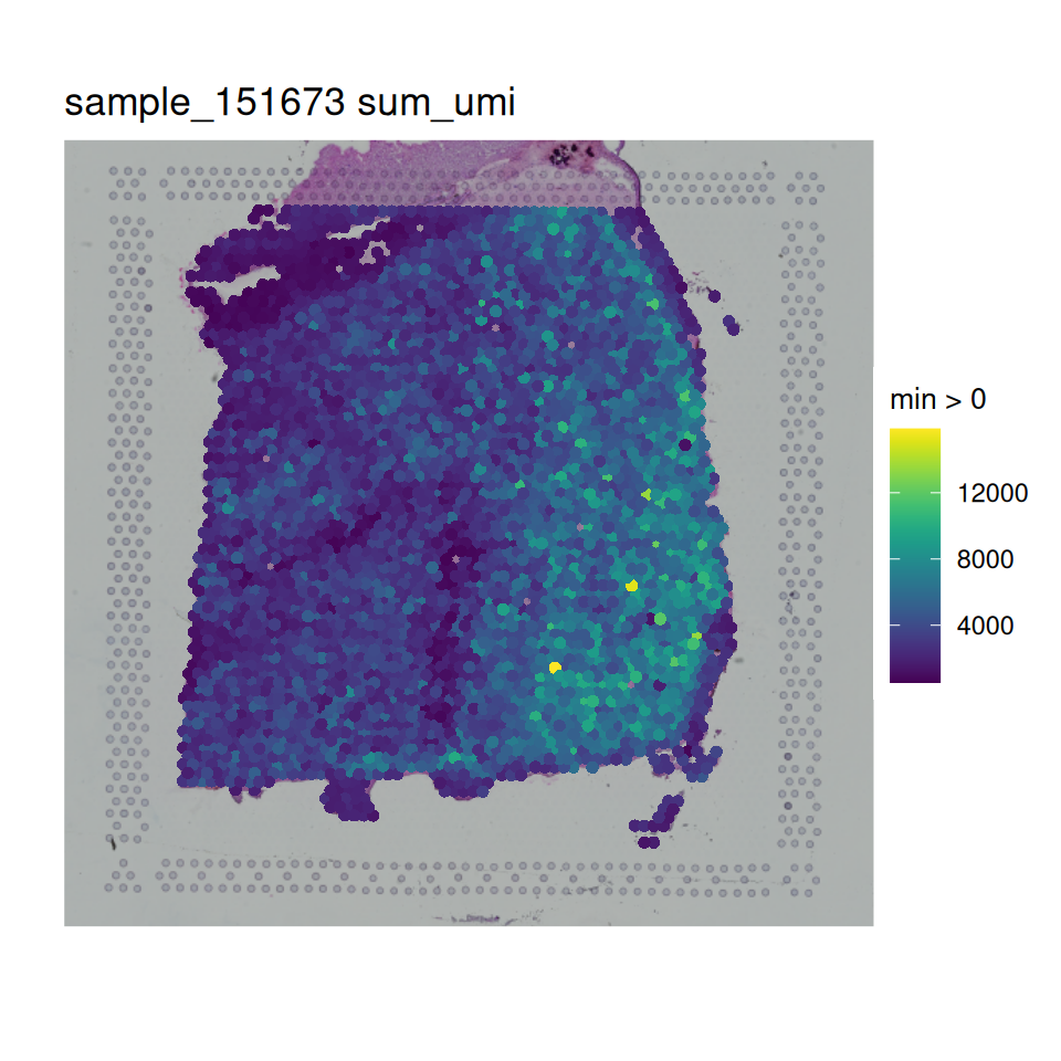
In order to visualize the data, we can then use spatialLIBD::vis_gene(). This is also a useful final check before we try launching our interactive website.

Code

# sum of UMI
spatialLIBD::vis_gene(
    spe = spe,
    sampleid = "sample_151673",
    geneid = "sum_umi"
)

Code

# PCP4 (layer 5 marker gene)
spatialLIBD::vis_gene(
    spe = spe,
    sampleid = "sample_151673",
    geneid = rowData(spe)$gene_search[which(rowData(spe)$gene_name == "PCP4")]
)

Now, let’s proceed to visualize the data interactively with a spatialLIBD-powered website. We have a number of variables to choose from. We will specify which are the continuous and discrete variables in our spatialLIBD::run_app() call.

Code

# explore all the variables we can use
colData(spe)

##  DataFrame with 3614 rows and 26 columns
##                             barcode_id     sample_id in_tissue array_row
##                            <character>   <character> <integer> <integer>
##  AAACAAGTATCTCCCA-1 AAACAAGTATCTCCCA-1 sample_151673         1        50
##  AAACAATCTACTAGCA-1 AAACAATCTACTAGCA-1 sample_151673         1         3
##  AAACACCAATAACTGC-1 AAACACCAATAACTGC-1 sample_151673         1        59
##  AAACAGAGCGACTCCT-1 AAACAGAGCGACTCCT-1 sample_151673         1        14
##  AAACAGCTTTCAGAAG-1 AAACAGCTTTCAGAAG-1 sample_151673         1        43
##  ...                               ...           ...       ...       ...
##  TTGTTTCACATCCAGG-1 TTGTTTCACATCCAGG-1 sample_151673         1        58
##  TTGTTTCATTAGTCTA-1 TTGTTTCATTAGTCTA-1 sample_151673         1        60
##  TTGTTTCCATACAACT-1 TTGTTTCCATACAACT-1 sample_151673         1        45
##  TTGTTTGTATTACACG-1 TTGTTTGTATTACACG-1 sample_151673         1        73
##  TTGTTTGTGTAAATTC-1 TTGTTTGTGTAAATTC-1 sample_151673         1         7
##                     array_col ground_truth   reference cell_count       sum
##                     <integer>  <character> <character>  <integer> <numeric>
##  AAACAAGTATCTCCCA-1       102       Layer3      Layer3          6      8458
##  AAACAATCTACTAGCA-1        43       Layer1      Layer1         16      1667
##  AAACACCAATAACTGC-1        19           WM          WM          5      3769
##  AAACAGAGCGACTCCT-1        94       Layer3      Layer3          2      5433
##  AAACAGCTTTCAGAAG-1         9       Layer5      Layer5          4      4278
##  ...                      ...          ...         ...        ...       ...
##  TTGTTTCACATCCAGG-1        42           WM          WM          3      4324
##  TTGTTTCATTAGTCTA-1        30           WM          WM          4      2761
##  TTGTTTCCATACAACT-1        27       Layer6      Layer6          3      2322
##  TTGTTTGTATTACACG-1        41           WM          WM         16      2331
##  TTGTTTGTGTAAATTC-1        51       Layer2      Layer2          5      6281
##                      detected subsets_mito_sum subsets_mito_detected
##                     <integer>        <numeric>             <integer>
##  AAACAAGTATCTCCCA-1      3586             1407                    13
##  AAACAATCTACTAGCA-1      1150              204                    11
##  AAACACCAATAACTGC-1      1960              430                    13
##  AAACAGAGCGACTCCT-1      2424             1316                    13
##  AAACAGCTTTCAGAAG-1      2264              651                    12
##  ...                      ...              ...                   ...
##  TTGTTTCACATCCAGG-1      2170              370                    12
##  TTGTTTCATTAGTCTA-1      1560              314                    12
##  TTGTTTCCATACAACT-1      1343              476                    13
##  TTGTTTGTATTACACG-1      1420              308                    12
##  TTGTTTGTGTAAATTC-1      2927              991                    13
##                     subsets_mito_percent     total qc_lib_size qc_detected
##                                <numeric> <numeric>   <logical>   <logical>
##  AAACAAGTATCTCCCA-1              16.6351      8458       FALSE       FALSE
##  AAACAATCTACTAGCA-1              12.2376      1667       FALSE       FALSE
##  AAACACCAATAACTGC-1              11.4089      3769       FALSE       FALSE
##  AAACAGAGCGACTCCT-1              24.2223      5433       FALSE       FALSE
##  AAACAGCTTTCAGAAG-1              15.2174      4278       FALSE       FALSE
##  ...                                 ...       ...         ...         ...
##  TTGTTTCACATCCAGG-1              8.55689      4324       FALSE       FALSE
##  TTGTTTCATTAGTCTA-1             11.37269      2761       FALSE       FALSE
##  TTGTTTCCATACAACT-1             20.49957      2322       FALSE       FALSE
##  TTGTTTGTATTACACG-1             13.21321      2331       FALSE       FALSE
##  TTGTTTGTGTAAATTC-1             15.77774      6281       FALSE       FALSE
##                       qc_mito   discard sizeFactor    label
##                     <logical> <logical>  <numeric> <factor>
##  AAACAAGTATCTCCCA-1     FALSE     FALSE   1.834415        4
##  AAACAATCTACTAGCA-1     FALSE     FALSE   0.361548        6
##  AAACACCAATAACTGC-1     FALSE     FALSE   0.817440        1
##  AAACAGAGCGACTCCT-1     FALSE     FALSE   1.178338        2
##  AAACAGCTTTCAGAAG-1     FALSE     FALSE   0.927835        4
##  ...                      ...       ...        ...      ...
##  TTGTTTCACATCCAGG-1     FALSE     FALSE   0.937812        1
##  TTGTTTCATTAGTCTA-1     FALSE     FALSE   0.598820        1
##  TTGTTTCCATACAACT-1     FALSE     FALSE   0.503608        5
##  TTGTTTGTATTACACG-1     FALSE     FALSE   0.505559        7
##  TTGTTTGTGTAAATTC-1     FALSE     FALSE   1.362256        2
##                                        key   sum_umi  sum_gene expr_chrM
##                                <character> <numeric> <integer> <numeric>
##  AAACAAGTATCTCCCA-1 sample_151673_AAACAA..      7051      3573         0
##  AAACAATCTACTAGCA-1 sample_151673_AAACAA..      1463      1139         0
##  AAACACCAATAACTGC-1 sample_151673_AAACAC..      3339      1947         0
##  AAACAGAGCGACTCCT-1 sample_151673_AAACAG..      4117      2411         0
##  AAACAGCTTTCAGAAG-1 sample_151673_AAACAG..      3627      2252         0
##  ...                                   ...       ...       ...       ...
##  TTGTTTCACATCCAGG-1 sample_151673_TTGTTT..      3954      2158         0
##  TTGTTTCATTAGTCTA-1 sample_151673_TTGTTT..      2447      1548         0
##  TTGTTTCCATACAACT-1 sample_151673_TTGTTT..      1846      1330         0
##  TTGTTTGTATTACACG-1 sample_151673_TTGTTT..      2023      1408         0
##  TTGTTTGTGTAAATTC-1 sample_151673_TTGTTT..      5290      2914         0
##                     expr_chrM_ratio ManualAnnotation
##                           <numeric>      <character>
##  AAACAAGTATCTCCCA-1               0               NA
##  AAACAATCTACTAGCA-1               0               NA
##  AAACACCAATAACTGC-1               0               NA
##  AAACAGAGCGACTCCT-1               0               NA
##  AAACAGCTTTCAGAAG-1               0               NA
##  ...                            ...              ...
##  TTGTTTCACATCCAGG-1               0               NA
##  TTGTTTCATTAGTCTA-1               0               NA
##  TTGTTTCCATACAACT-1               0               NA
##  TTGTTTGTATTACACG-1               0               NA
##  TTGTTTGTGTAAATTC-1               0               NA

Code

# run our shiny app
if (interactive()) {
    spatialLIBD::run_app(
        spe,
        sce_layer = NULL,
        modeling_results = NULL,
        sig_genes = NULL,
        title = "OSTA spatialLIBD workflow example",
        spe_discrete_vars = c("ground_truth", "label", "ManualAnnotation"),
        spe_continuous_vars = c(
            "cell_count",
            "sum_umi",
            "sum_gene",
            "expr_chrM",
            "expr_chrM_ratio",
            "sum",
            "detected",
            "subsets_mito_sum",
            "subsets_mito_detected",
            "subsets_mito_percent",
            "total",
            "sizeFactor"
        ),
        default_cluster = "label"
    )
}

Screenshot of the ‘clusters (interactive)’ section of the ‘spot-level data’ panel created with with the data from this workflow.

11.3.6 Sharing your website

Now that you have created a spatialLIBD-powered website, you might be interested in sharing it. To do so, it will be useful to save a small spe object using saveRDS(), containing the data to share. The smaller the object, the better in terms of performance. For example, you may want to remove lowly expressed genes to save space. You can check the object size in R with object.size().

Code

# object size
format(object.size(spe), units = "MB")

##  [1] "308.1 Mb"

If your data is small enough, you might want to share your website by hosting on shinyapps.io by Posit (the company that develops RStudio), which you can try for free. Once you have created your account, you need to create an app.R file like the one we have on the spatialLIBD_demo directory.

##  library("spatialLIBD")
##   library("markdown") # for shinyapps.io
##   
##   ## spatialLIBD uses golem
##   options("golem.app.prod" = TRUE)
##   
##   ## You need this to enable shinyapps to install Bioconductor packages
##   options(repos = BiocManager::repositories())
##   
##   ## Load the data
##   spe <- readRDS("spe_workflow_Visium_spatialLIBD.rds")
##   
##   ## Deploy the website
##   spatialLIBD::run_app(
##       spe,
##       sce_layer = NULL,
##       modeling_results = NULL,
##       sig_genes = NULL,
##       title = "OSTA spatialLIBD workflow example",
##       spe_discrete_vars = c("ground_truth", "label", "ManualAnnotation"),
##       spe_continuous_vars = c(
##           "cell_count",
##           "sum_umi",
##           "sum_gene",
##           "expr_chrM",
##           "expr_chrM_ratio",
##           "sum",
##           "detected",
##           "subsets_mito_sum",
##           "subsets_mito_detected",
##           "subsets_mito_percent",
##           "total",
##           "sizeFactor"
##       ),
##       default_cluster = "label",
##       docs_path = "www"
##   )

You can then open R in a new session in the same directory where you saved the app.R file, run the code and click on the “publish” blue button at the top right of your RStudio window. You will then need to upload the app.R file, your .rds file containing the spe object, and the files under the www directory which enable you to customize your spatialLIBD website.

Screenshot of the RStudio window for publishing your spatialLIBD-powered website to shinyapps.io

The RStudio prompts will guide you along the process for authenticating to your shinyapps.io account, which will involve copy-pasting some code that starts with rsconnect::setAccountInfo(). Alternatively, you can create a deploy.R script and write the code for uploading your files to shinyapps.io as shown below.

##  library('rsconnect')
##   
##   ## Or you can go to your shinyapps.io account and copy this
##   ## Here we do this to keep our information hidden.
##   # load(".deploy_info.Rdata")
##   # rsconnect::setAccountInfo(
##   #     name = deploy_info$name,
##   #     token = deploy_info$token,
##   #     secret = deploy_info$secret
##   # )
##   
##   ## You need this to enable shinyapps to install Bioconductor packages
##   options(repos = BiocManager::repositories())
##   
##   ## Deploy the app, that is, upload it to shinyapps.io
##   rsconnect::deployApp(
##       appFiles = c(
##           "app.R",
##           "spe_workflow_Visium_spatialLIBD.rds",
##           dir("www", full.names = TRUE)
##       ),
##       appName = 'OSTA_spatialLIBD_demo',
##       account = 'libd',
##       server = 'shinyapps.io'
##   )

Note that we have copied the default www directory files from the spatialLIBD repository and adapted them. We then use these files with spatialLIBD::run_app(docs_path) in our app.R script. These files help us control portions of our spatialLIBD-powered website and customize it.

If you follow this workflow, you will end up with a website just like this one. In our case, we further configured our website through the shinyapps.io dashboard. We selected the following options:

General Instance Size: 3X-Large (8GB)
Advanced Max Worker Processes: 1
Advanced Max Connections: 15

The Max Worker Processes determines how many R sessions are open per instance. Then Max Connections specifies the number of connections to each R session. The Instance Size determines the memory available. In this case, 8000 / 300 is approximately 27, but we decided to be conservative and set the total number of users per instance to 15. This is why it can be important to reduce the size of your spe object before sharing the website. Alternatively, you can rent an AWS Instance and deploy your app there, which is how http://spatial.libd.org/spatialLIBD is hosted along with these error configuration files.

11.3.7 Wrapping up

Thank you for reading this far! In this section we showed you:

why you might be interested in using spatialLIBD,
we re-used the spe object from the DLPFC workflow (Section 11.2),
we adapted the spe object to make it compatible with spatialLIBD,
we created an interactive website on our laptops,
we shared the website with others using shinyapps.io.

11.4 Appendix

References

Lun, Aaron T. L., Davis J. McCarthy, and John C. Marioni. 2016. “A Step-by-Step Workflow for Low-Level Analysis of Single-Cell RNA-seq Data with Bioconductor.” F1000Research 5 (2122). https://doi.org/10.12688/f1000research.9501.2.

Maynard, Kristen R., Leonardo Collado-Torres, Lukas M. Weber, Cedric Uytingco, Brianna K. Barry, Stephen R. Williams, Joseph L. Catallini II, et al. 2021. “Transcriptome-Scale Spatial Gene Expression in the Human Dorsolateral Prefrontal Cortex.” Nature Neuroscience 24: 425–36. https://doi.org/10.1038/s41593-020-00787-0.

McCarthy, Davis J., Kieran R. Campbell, Aaron T. L. Lun, and Quin F. Wills. 2017. “Scater: Pre-Processing, Quality Control, Normalization and Visualization of Single-Cell RNA-seq Data in R.” Bioinformatics 33 (8): 1179–86. https://doi.org/10.1093/bioinformatics/btw777.

Pardo, Brenda, Abby Spangler, Lukas M. Weber, Stephanie C. Page, Stephanie C. Hicks, Andrew E. Jaffe, Keri Martinowich, Kristen R. Maynard, and Leonardo Collado-Torres. 2022. “spatialLIBD: An R/Bioconductor Package to Visualize Spatially-Resolved Transcriptomics Data.” BMC Genomics, no. 23: 434. https://doi.org/10.1186/s12864-022-08601-w.

Weber, Lukas M., Arkajyoti Saha, Abhirup Datta, Kasper D. Hansen, and Stephanie C. Hicks. 2023. “nnSVG for the Scalable Identification of Spatially Variable Genes Using Nearest-Neighbor Gaussian Processes.” Nature Communications 14: 4059. https://doi.org/10.1038/s41467-023-39748-z.