3  Interoperability

3.1 Introduction

Ideally, users would be able to leverage the full range of available tools for their analysis. Methods should be selected based on scientific merit (as demonstrated by third-party benchmarks), and independent of having been implemented in a given programming language (R or Python) or framework (say, Bioconductor or Seurat).

For single-cell and spatial omics data analysis, being able to leverage different ecosystems is especially powerful. On the one hand, Python offers superb infrastructure for image analysis and machine learning-based approaches. On the other hand, the R programming language has been historically dedicated to statistical computing; as a result, many a modern R method for spatial omics data builds on a solid foundation of tools for spatial statistics and statistical modeling in general.

R’s application to spatial data dates back decades, primarily in epidemiological and geospatial research. As a result, various tools for spatial analyses have been established; for example, sp provides a “coherent set of classes and methods for […] points, lines, polygons, and grids”; spatstat and, more recently, sf provide tools for spatial point pattern and vector data, respectively.

Different data structures, although standardized within a given framework, make switching between languages and tools especially cumbersome. In the realm of single-cell and spatial omics, Bioconductor tools build around SummarizedExperiment-derived classes, while Seurat, Giotto and VoltRon rely on objects built in-house; and Python’s scanpy (Wolf, Angerer, and Theis 2018) and squidpy (Palla et al. 2022) use AnnData. Attempts to alleviate the problem are being made; e.g. zellkonverter and functions from Seurat allow for conversion between Python’s AnnData, R/Bioconductor’s SingleCellExperiment and also SingleCellExperiment.

On a higher level, tools that enable interoperability between programming languages have become available. For example, the reticulate package provides an R interface to Python, including support to translate between objects from both languages; basilisk facilitates Python environment management within the Bioconductor ecosystems, but can be interfaced with reticulate as well; and, Quarto can generate dynamic reports from code in different languages.

Quarto is the successor of R Markdown by Posit (formerly known as RStudio). Similar to .rmd files, .qmd files can include scientific content (e.g. cross-referencing, LaTeX-based equations), and can be published in multiple output formats (HTML, PDF, etc.). – This book uses Quarto.

3.2 Dependencies

library(OSTA.data)
library(SpatialExperiment)
library(VisiumIO)
library(zellkonverter)
library(jsonlite)
library(reticulate)
library(basilisk)

3.3 Configuring Python

We first create an environment with Python modules necessary for the examples in this chapter. For that, we first define a basilisk environment and use the resulting conda environment with reticulate.

env <- BasiliskEnvironment(
  envname="bkg-interop", 
  pkgname="base",
  channels=c("conda-forge", "bioconda", "pytorch"),
  packages=c(
    "python=3.11",
    "Dask=2024.12.1"),
  pip=c(
    "squidpy==1.6.2"))
use_virtualenv(obtainEnvironmentPath(env))

##  Installing pyenv ...
##  Done! pyenv has been installed to '/root/.local/share/r-reticulate/pyenv/bin/pyenv'.
##  Using Python: /root/.pyenv/versions/3.11.12/bin/python3.11
##  Creating virtual environment '/root/.cache/R/basilisk/1.21.5/base/4.5.0/bkg-interop' ...

##  + /root/.pyenv/versions/3.11.12/bin/python3.11 -m venv /root/.cache/R/basilisk/1.21.5/base/4.5.0/bkg-interop

##  Done!
##  Installing packages: pip, wheel, setuptools

##  + /root/.cache/R/basilisk/1.21.5/base/4.5.0/bkg-interop/bin/python -m pip install --upgrade pip wheel setuptools

##  Installing packages: 'Dask==2024.12.1', 'squidpy==1.6.2'

##  + /root/.cache/R/basilisk/1.21.5/base/4.5.0/bkg-interop/bin/python -m pip install --upgrade --no-user 'Dask==2024.12.1' 'squidpy==1.6.2'

##  Virtual environment '/root/.cache/R/basilisk/1.21.5/base/4.5.0/bkg-interop' successfully created.

3.4 SingleCellExperiment

3.4.1 Calling Python

After configuring the python environment, R commands will now be reticulated; e.g.:

Note that running code in this way comes with the overhead of starting up a Python session in the background. But this is typically negligible compared to the runtime required to run computation-heavy methods, or when analyzing large-scale single-cell and spatial data (100,000s of cells).

anndata <- reticulate::import("anndata")
example_h5ad <- system.file("extdata", "krumsiek11.h5ad", package = "zellkonverter")
(ad <- anndata$read_h5ad(example_h5ad))

##  AnnData object with n_obs × n_vars = 640 × 11
##      obs: 'cell_type'
##      uns: 'highlights', 'iroot'

3.4.2 Continuing in R

We can access any of the variables above in R. For basic outputs, this works out of the box:

unique(ad$obs$cell_type)

##  [1] progenitor Mo         Ery        Mk         Neu       
##  Levels: Ery Mk Mo Neu progenitor

Then again, reticulate supports few direct type conversions (e.g. dictionary \(\leftrightarrow\) named list). In the example demonstrated here, we can use zellkonverter to go from AnnData to SingleCellExperiment:

(sce <- AnnData2SCE(ad))

##  class: SingleCellExperiment 
##  dim: 11 640 
##  metadata(2): highlights iroot
##  assays(1): X
##  rownames(11): Gata2 Gata1 ... EgrNab Gfi1
##  rowData names(0):
##  colnames(640): 0 1 ... 158-3 159-3
##  colData names(1): cell_type
##  reducedDimNames(0):
##  mainExpName: NULL
##  altExpNames(0):

3.4.3 Back to Python

We can also do the reverse, i.e. go from R’s SingleCellExperiment to Python’s AnnData:

(ad <- SCE2AnnData(sce, X_name="X"))

##  AnnData object with n_obs × n_vars = 640 × 11
##      obs: 'cell_type'
##      uns: 'X_name', 'highlights', 'iroot'

3.5 SpatialExperiment

Since SpatialExperiment extends the SingleCellExperiment class, conversion operations that we discussed above are also applicable to the SpatialExperiment class. However, to accomplish a full conversion from the AnnData object, we need to manually insert/import the remaining spatial information using reticulate directly.

3.5.1 Starting with R

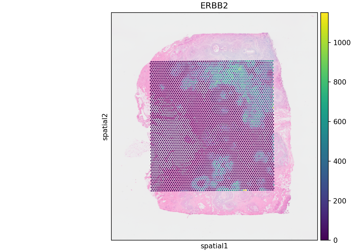
For this use case with SpatialExperiment, we will use the dataset from Janesick et al. (2023), which includes Visium measurements on human breast cancer tissue.

id <- "Visium_HumanBreast_Janesick"
pa <- OSTA.data_load(id)
dir.create(td <- tempfile())
unzip(pa, exdir=td)
obj <- TENxVisium(
    spacerangerOut=td, 
    format="h5", 
    images="lowres")
(spe <- VisiumIO::import(obj))

We also have to parse the original scaling information (i.e. scale factor) for spots and images available in standard Visium output. We will use this later during conversion.

scalefactors <- jsonlite::read_json(file.path(td, "outs/spatial/scalefactors_json.json"))

We again use the SCE2AnnData function from the previous example, and convert the SingleCellExperiment relevant components of the SpatialExperiment object to an AnnData object.

(ad <- SCE2AnnData(spe, X_name="counts"))

##  AnnData object with n_obs × n_vars = 4992 × 18085
##      obs: 'in_tissue', 'array_row', 'array_col', 'sample_id'
##      var: 'ID', 'Symbol', 'Type'
##      uns: 'X_name', 'resources', 'spatialList'
##      obsm: 'spatial'

We should now populate uns and obsm components of AnnData with spatial coordinates and images. We start with the coordinates.

coords <- spatialCoords(spe)
colnames(coords) <- c("x", "y")
obsm <- list(spatial = coords)

Now lets create the uns component. The list of uns should compose of as many samples as the images in the SpatialExperiment object. Also, each sample entry in the list should have two elements, one for the image and the other for scaling information.

# get image metadata
imgdata <- imgData(spe)

# get image
img <- imgRaster(spe)
img <- apply(img, c(1,2), \(x) col2rgb(x))
img <- aperm(img, perm = c(2,3,1))
img <- img/255

# create uns
uns <- list(
  spatial = setNames(list(NULL), imgdata$sample_id)
)
uns[["spatial"]][[imgdata$sample_id]] <-
  list(images = list(lowres = img),
       scalefactors = scalefactors)

Now lets insert the components to the AnnData object, and write back to an h5ad file.

ad$obs$library_id <- imgdata$sample_id
ad$obsm <- obsm
ad$uns <- uns
ad$write_h5ad("spe.h5ad")

3.5.2 Calling Python

Now that we have converted our SpatialExperiment object to AnnData format, we visualize the Visium data using, for example, the squidpy module.

import squidpy as sq
import anndata as ad
import matplotlib.pyplot as plt

Now, we read spe.h5ad and visualize features and/or gene expression (e.g. ERBB2).

adata = ad.read_h5ad("spe.h5ad")
adata.var_names = adata.var['Symbol'].astype(str)
sq.pl.spatial_scatter(adata,
                      color=["ERBB2"], 
                      img_res_key = "lowres")

3.6 Appendix

References

Janesick, Amanda, Robert Shelansky, Andrew D. Gottscho, Florian Wagner, Stephen R. Williams, Morgane Rouault, Ghezal Beliakoff, et al. 2023. “High Resolution Mapping of the Tumor Microenvironment Using Integrated Single-Cell, Spatial and in Situ Analysis.” Nature Communications 14 (1): 8353.

Palla, Giovanni, Hannah Spitzer, Michal Klein, David Fischer, Anna Christina Schaar, Louis Benedikt Kuemmerle, Sergei Rybakov, et al. 2022. “Squidpy: A Scalable Framework for Spatial Omics Analysis.” Nature Methods 19 (2): 171–78.

Wolf, F Alexander, Philipp Angerer, and Fabian J Theis. 2018. “SCANPY: Large-Scale Single-Cell Gene Expression Data Analysis.” Genome Biology 19 (1): 15.