In single-cell omics data analysis, dimension reduction (DR) techniques are often categorized as linear (e.g., multi-dimensional scaling (MDS), linear discriminant analysis (LDA), principal component analysis (PCA)), or non-linear (e.g., t-distributed stochastic neighbor embedding (t-SNE), uniform manifold approximation and projection (UMAP)); see OSCA.
In the context of ST data, we would instead like to distinguish between spatially aware and non-spatial methods, i.e., whether or not DR incorporates physical locations or is based on molecular profiles only. Spatially aware DR may be used as input for standard single-cell clustering approaches (say, SNN-graph based Leiden), while non-spatial DR may be used for spatially aware clustering. While these approach may differ in methodological detail, they are arguably similar conceptually. We will try and demonstrate as much here.
# get annotations from 'BiocFileCache'# (data has been retrieved already)id<-"Xenium_HumanBreast1_Janesick"pa<-OSTA.data_load(id)dir.create(td<-tempfile())unzip(pa, "annotation.csv", exdir=td)df<-read.csv(list.files(td, full.names=TRUE))# add annotations as cell metadatacs<-match(spe$cell_id, df$Barcode)spe$Label<-df$Annotation[cs]
22.2 Principal component analysis (PCA)
22.2.1 Non-spatial
As a baseline, we will perform principal component analysis (PCA), which underlies many standard scRNA-seq analysis pipelines, such as (spatially unaware) graph-based clustering based on a shared nearest neighbor (SNN) graph and the Leiden or Louvain algorithm for community detection.
A standard approach is to apply PCA to the set of top HVGs, and retain a subset of PCs for subsequent steps. This is done for two main reasons: (i) to reduce noise due to random variation in expression of biologically uninformative genes, which are assumed to have expression patterns independent of each other, and (ii) to improve computational efficiency. Because our data are relatively low-plex in this example, we use all features instead.
For large-scale datasets (100,000s of cells), argument BSPARAM=RandomParam() can be used to decrease runtime by approximating the singular value decomposition (SVD). Because this implementation uses randomization, and seed for random number generation should be set in order to make results reproducible.
BANKSY(Singhal et al. 2024) computes PCs on a spatial-neighborhood augmented matrix, thereby embedding cells in a product space of their own and their local neighborhood’s (average) transcriptome, representing cell state and microenvironment. A key parameter for this method is \(\lambda\in[0,1]\) (argument lambda in runBanksyPCA()), which controls the spatial component’s weight; notably, when \(\lambda=0\), BANKSY reduces to non-spatial clustering. Secondly, k_geom determines the number of neighbors to use for computing local transcriptomic neighborhoods.
In Visium, \(k=6\) would correspond to first-order, \(k=18\) to first- and second-order neighbors.
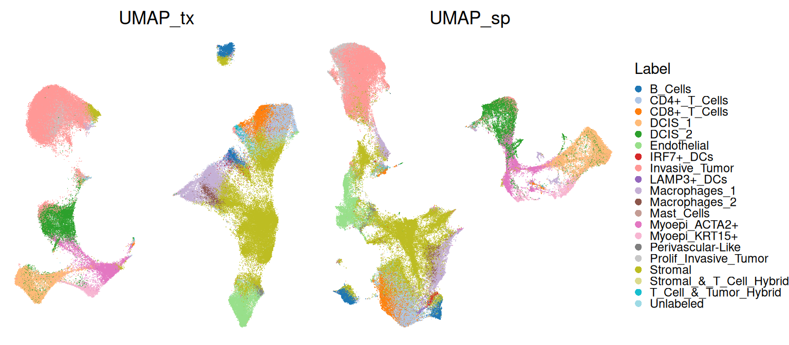
To not confuse different types of PCs, we rename the corresponding reducedDims to end in _sp and _tx for spatially aware and unaware results, respectively.
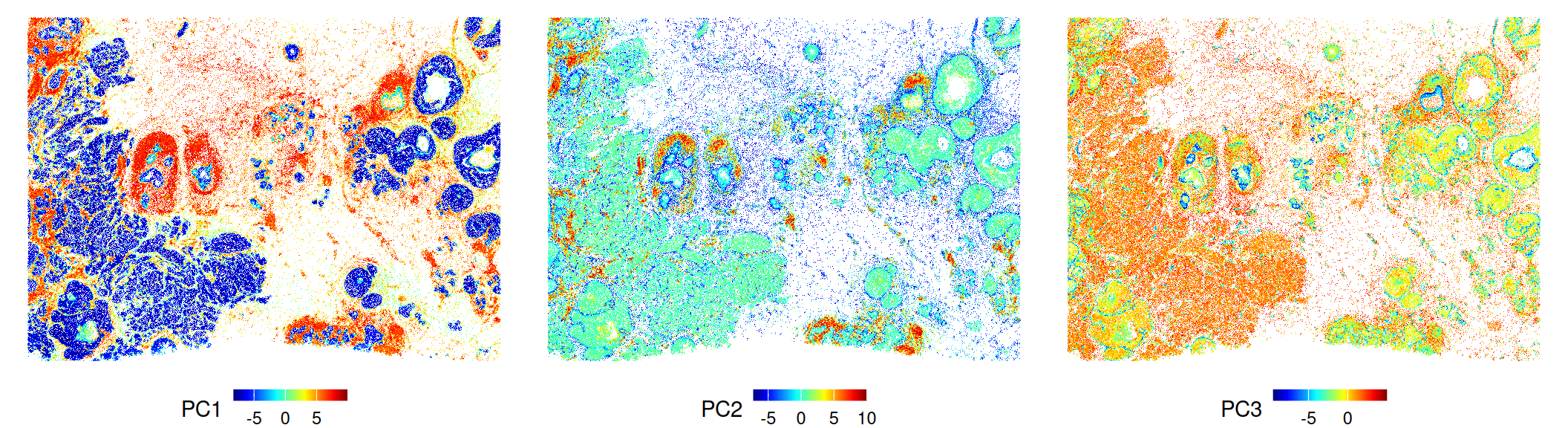
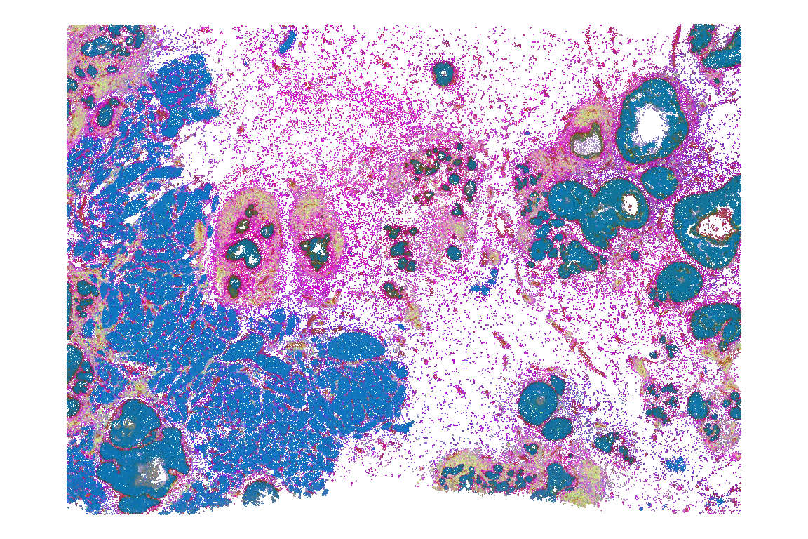
A useful visualization is to color cells by their PCs in physical space. This will help highlight key drivers of transcriptional variability, e.g., between major biological compartments such as epithelia, immune and stromal cells. Exemplary plots of PCs 1-3 are rendered below:
E.g., we see that colors corresponding to opposing PC values are clearly separated in space, indicating distinct drivers of transcriptional variability. In some regions, we see color mixtures, indicating cells of ambiguous transcriptional profiles (with respect to what is being captured by the 3 PCs considered here).
McCarthy, Davis J., Kieran R. Campbell, Aaron T. L. Lun, and Quin F. Wills. 2017. “Scater: Pre-Processing, Quality Control, Normalization and Visualization of Single-Cell RNA-seq Data in R.”Bioinformatics 33 (8): 1179–86. https://doi.org/10.1093/bioinformatics/btw777.
Singhal, Vipul, Nigel Chou, Joseph Lee, Yifei Yue, Jinyue Liu, Wan Kee Chock, Li Lin, et al. 2024. “BANKSY Unifies Cell Typing and Tissue Domain Segmentation for Scalable Spatial Omics Data Analysis.”Nature Genetics 56 (3): 431–41.