38 Spatial registration
38.1 Preamble
38.1.1 Introduction
Spatial registration is defined as the task of mapping features or spatial locations of observations from a query to a reference assay (Friston et al. 1995; Lewis et al. 2021; Nitzan et al. 2019). Here, the reference is a spatially-resolved dataset whereas the query could be an assay with or without spatial resolution.
In this chapter, we demonstrate methods that are available in R/Bioconductor for aligning (or registering) spatially-resolved datasets, where the utility and function of the alignment method is defined by the modality of the query dataset.
We will touch upon two cases: (1) alignment, where both reference and query data are spatially resolved; and, (2) reconstruction, where spatial information is inferred from non-spatial data.
38.1.2 Dependencies
In this demo, we will use the Xenium data generated from a human breast cancer biopsy (Janesick et al. 2023), which is available from OSTA.data (see Chapter 7):
Code
# retrieve dataset from OSF repo
id <- "Xenium_HumanBreast1_Janesick"
pa <- OSTA.data_load(id, mol=FALSE)
dir.create(td <- tempfile())
unzip(pa, exdir=td)
# read into 'SpatialExperiment'
xen <- readXeniumSXE(td, addTx=FALSE)
xen$sample_id <- "Xenium"
xen
## class: SpatialExperiment
## dim: 313 167780
## metadata(3): experiment.xenium cell_boundaries nucleus_boundaries
## assays(1): counts
## rownames(313): ABCC11 ACTA2 ... ZEB2 ZNF562
## rowData names(3): ID Symbol Type
## colnames(167780): 1 2 ... 167779 167780
## colData names(8): cell_id transcript_counts ... nucleus_area
## sample_id
## reducedDimNames(0):
## mainExpName: NULL
## altExpNames(4): NegControlProbe NegControlCodeword antisense BLANK
## spatialCoords names(2) : x_centroid y_centroid
## imgData names(1): sample_id38.2 Alignment
Spatial omic technologies often generate data modalities that capture morphological features of tissue sections as well as omic profiles of cells, spots or other types of observations. Localization of these profiles can also be defined in different units and even in different perspectives (i.e., coordinate systems). Image alignment and registration methods provide transformations to map spatial locations of observations from one coordinate system to another, thus allowing to transfer data across observations from identical tissue sections, adjacent sections, as well as sections with similar morphology and structure.
Strategies and approaches for aligning spatial omic assays differ depending on the modality and/or instrument used to generate these data. These methods could be categorized into two classes, where some incorporate (i) the morphology of microscopy images (image registration) of reference and query data (Friston et al. 1995) and others that rely on the (ii) spatial locations of observations (cells or spots) and the distribution of omic profiles (omics coverage) (Kiessling and Kuppe 2024).
38.2.1 Image-based
To facilitate alignment using images, we will showcase how to incorporate VoltRon to align a SpatialExperiment object of Xenium data with a post-Xenium hematoxylin and eosin (H&E) stain of the same tissue section.
The SpatialExperiment of the Xenium data does not include any images. To perform the spatial alignment via image registration, we first add an image of the corresponding DAPI staining to the object’s imgData.
The RBioFormats package can be used to read a specific resolution from multi-resolution ome.tiff image pyramids. Here, we choose the lowest resolution of the morphology_mip.ome.tif from the standard Xenium output. We also define the parameter (pixel-to-micron ratio) to scale the spatial coordinates of cells accordingly:
Code
res <- 7 # target resolution
px <- 0.2125 # px size (um)
sf <- px*(2^(res-1)) # scale factor
img <- RBioFormats::read.image(
    "morphology_mip.ome.tif",
    resolution=res)
Before adding the selected DAPI image to the SpatialExperiment object, we first normalize the contrast to 1, and then save the image to a temporary .png file:
Code
img <- img/max(img)
png <- "Xenium_DAPI_res7.png"
EBImage::writeImage(img, files=png, type="png")
We can now add the DAPI channel to the SpatialExperiment object:
Code
## DataFrame with 1 row and 4 columns
## sample_id image_id data scaleFactor
## <character> <character> <list> <numeric>
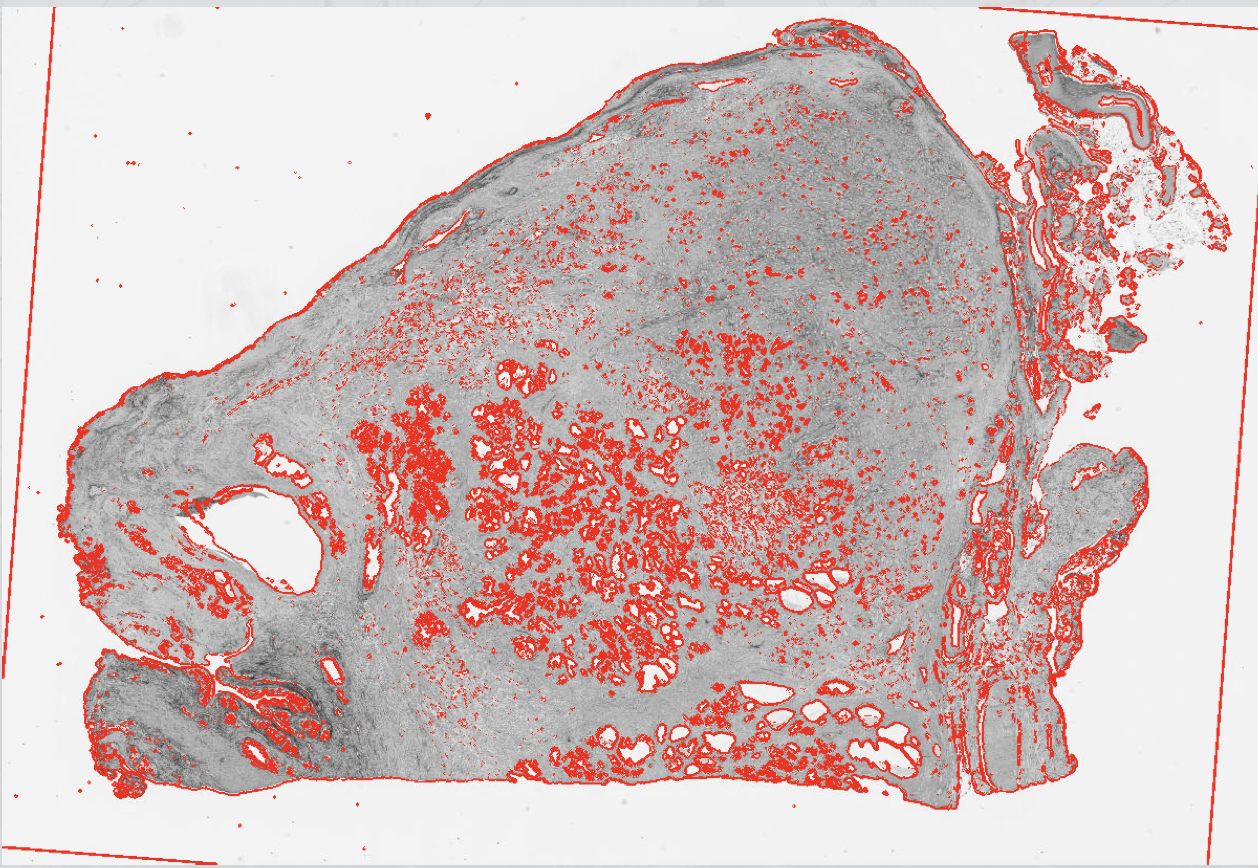
## 1 Xenium DAPI #### 0.0735294Let’s visualize the new DAPI image and overlay with cell centroids using ggspavis:
Code
# plot DAPI image
p <- plotVisium(xen, spots=FALSE, image_id="DAPI")
# overlay cells with image
img <- imgRaster(xen)
sf <- scaleFactors(xen)
xy <- spatialCoords(xen)*sf
xy[, 2] <- nrow(img)-xy[, 2]
p + geom_point(
    aes(x_centroid, y_centroid), data.frame(xy),
    shape=16, stroke=0, size=0.2, alpha=0.4,
col="red", inherit.aes=FALSE) 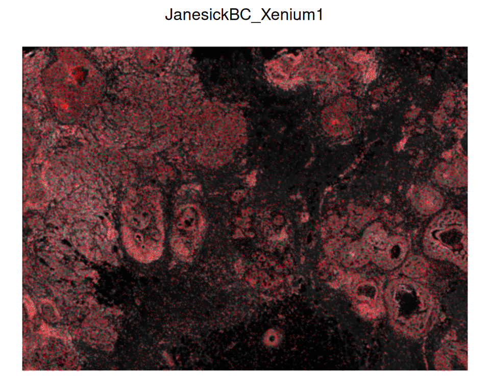
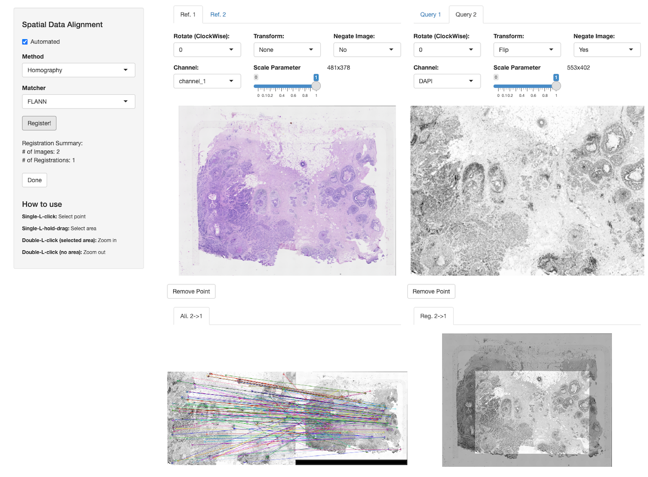
At this stage, one may use VoltRon (or another tool) in order to register the query spatial data onto the reference (in this example, query = cell centroids, reference = H&E staining).
The return value of VoltRon’s registerSpatialData() function includes an affine transformation matrix that may be used to register spatial coordinates:
An affine map is generally composed of a linear map (scaling and rotation) and a translation, and can be apply using basic matrix multiplication and vector addition, specifically:
\[\mathbf{y}=A\mathbf{x}+\mathbf{b}\]
where \(A\) denotes the linear map, \(b\) the translation, and \(\mathbf{x}\) and \(\mathbf{y}\) correspond to original and transformed coordinates, respectively.
In R, this translates to the following operations:
Code
img <- imgRaster(xen)
xy <- spatialCoords(xen)
xy <- xy*scaleFactors(xen)
xy[, 2] <- nrow(img) - xy[, 2]
xy_reg <- t(mtx %*% rbind(t(xy), 1))
xy_reg <- xy_reg[, -3]
colnames(xy_reg) <- colnames(spatialCoords(xen))
# create a dataset copy with new coordinates
reg <- xen
imgData(reg) <- NULL
spatialCoords(reg) <- xy_reg
Now that the registered Xenium data and the post-Xenium H&E image have identical coordinate systems, we can add the H&E image directly to the registered SpatialExperiment object:
Code
tif <- "GSM7780153_Post-Xenium_HE_Rep1.ome.tif"
img <- RBioFormats::read.image(tif, resolution=7)
png <- "Xenium_H&E_res7.png"
EBImage::writeImage(tif, files=png, type="png")
Code
##  DataFrame with 1 row and 4 columns
##      sample_id    image_id   data scaleFactor
##    <character> <character> <list>   <numeric>
##  1      Xenium         H&E   ####           1
Again, we can visualize the registered Xenium cells on the H&E image:
Code
# plot H&E image
p <- plotVisium(reg, spots=FALSE, image_ids="H&E")
# overlay cells with image
img <- imgRaster(reg)
sf <- scaleFactors(reg)
xy <- spatialCoords(reg)*sf
xy[, 2] <- nrow(img)-xy[, 2]
p + geom_point(
    aes(x_centroid, y_centroid), data.frame(xy),
    shape=16, stroke=0, size=0.2, alpha=0.4,
    col="red", inherit.aes=FALSE)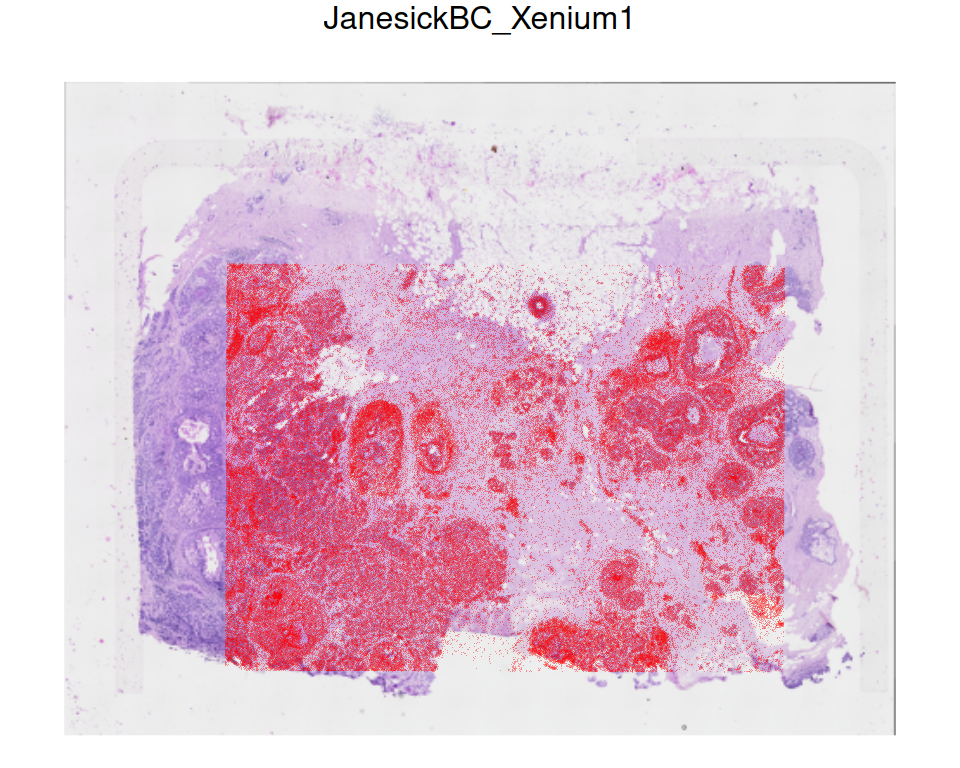
A number of R/Python frameworks can be used to automatically or manually align microscopy images associated with spatial omics datasets. The Python modules could be used through R packages such as reticulate and basilisk.
- VoltRon (Manukyan et al. 2023) is an R package that allows alignment between multiple spatially aware datasets of distinct modalities. A Shiny application is provided to enable both automated and manual alignment across adjacent/same tissue sections where users can interactively manipulate microscopy images and choose landmark points for co-registration.
-
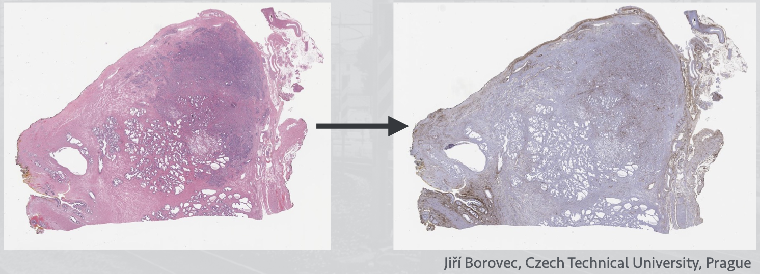
RNiftyReg is an R wrapper package, and can be combined with mmand for automated image registration using both rigid and non-rigid approaches. Users can extract and apply the resulting transformation matrix on spatial coordinates of a
SpatialExperimentobject. However, the automation does not work well on images with very different orientation, scale, and intensity (e.g., Xenium and Visium; see also Chapter 40). Here is a demonstration with external data, before and after registration of the two slices:
STalign (Clifton et al. 2023) is a Python module that performs optimal transport across two sets of spatial coordinates with or without associated microscopy images. Rasterization of spatial coordinates could be performed when the one of either query and reference assay missing any background microscopy images with, e.g. H&E and/or DAPI staining.
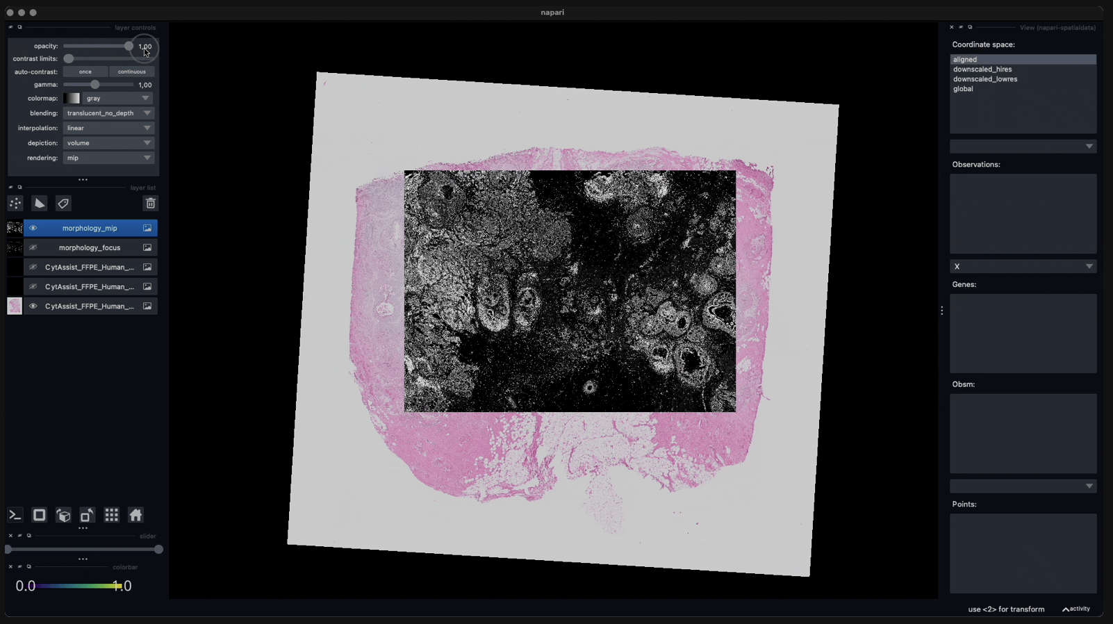
spatialdata (Marconato et al. 2025) is a Python framework, maintained by the scverse consortium. Combined with the napari platform,
spatialdataallows users to manually select landmark points before performing rigid alignment between two objects. Here we show the registration of Visium onto Xenium in napari:
38.2.2 Omics-based
Spatial alignment approaches that depend only on the spatial distribution of omic profiles are mostly available in Python frameworks which could be used in R through packages such as reticulate and basilisk.
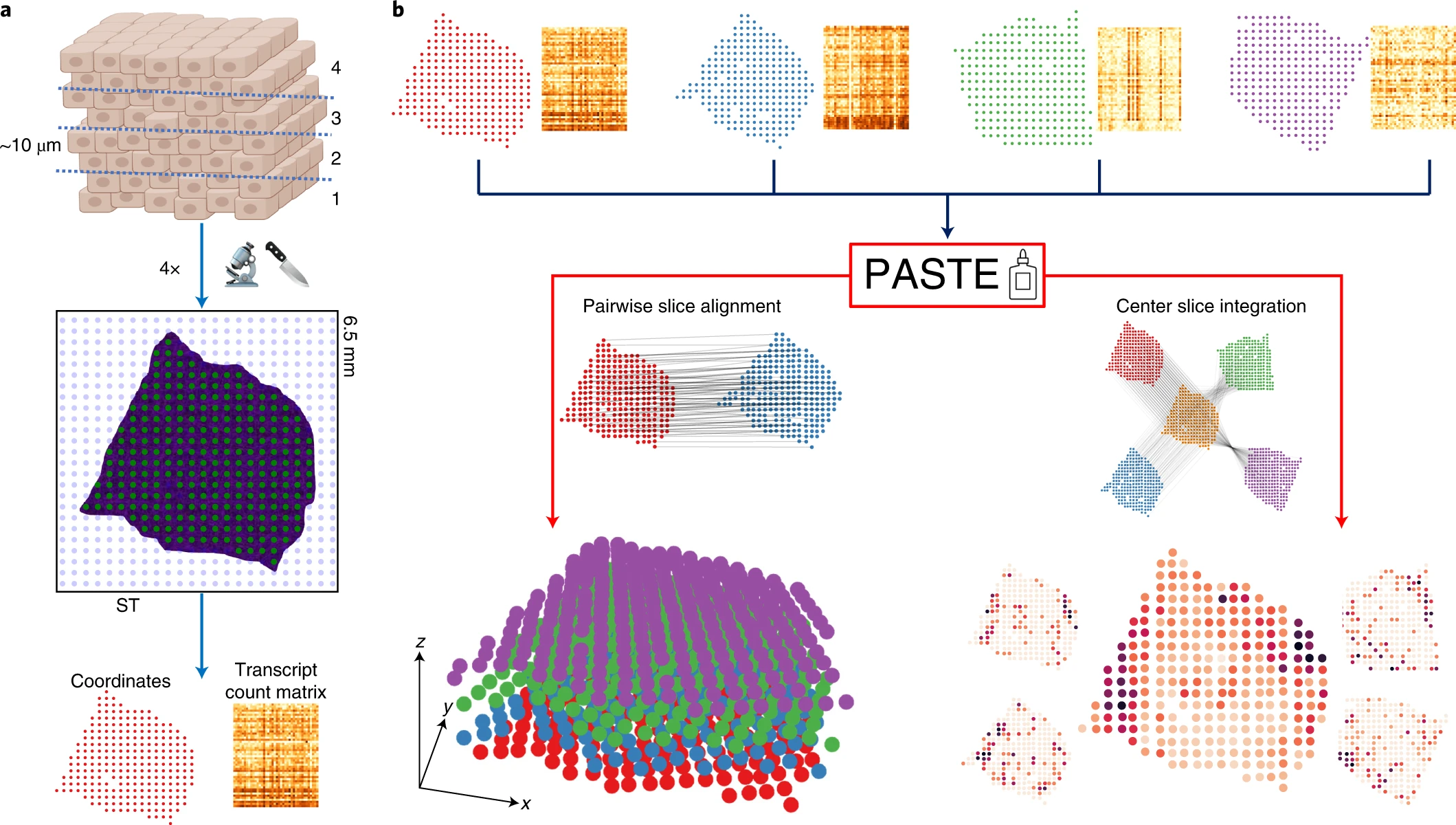
- PASTE is a Python-based framework (Zeira et al. 2022) that perform pairwise alignment between serial sections by solving a fused Gromov–Wasserstein optimal transport problem. The solution finds a mapping between each pair of adjacent slices by minimizing a transport cost that depends on both gene expression profiles and distance between spots of each slice.
- SLAT is another alternative provided as a Python module scSLAT (Xia et al. 2023) that jointly models spatial coordinates and omics features using spatial graph with node embeddings. Here, the node embeddings are generated by batch-corrected embeddings of omics features whereas the graph is constructed using edges detected by either kNN or radial neighbors. The solution is found by minimizing the cost of a bipartite matching problem.
38.3 Reconstruction
We now move to the second case where the query dataset includes no spatial information, and where we instead would like to leverage spatially-resolved reference data in order to ‘reconstruct’ the spatial coordinates of query single cells.
Below we give a list of Python frameworks that reconstruct the spatial locations of single-cell profiles. Some of these methods could be used through R using packages such as reticulate and basilisk.
CeLEry (Zhang et al. 2023) incorporates a supervised deep neural network model to learn the relationship between spot/cell profiles of spatial omics data and associated localization information, and then uses this model to predict the localization of single cell profiles by using the scRNA-seq data as input.
novosparc (Nitzan et al. 2019) utilizes optimal transport (OT) to find a probabilistic embedding between expression space and physical space of single cells that minimizes the discrepancy between the pairwise graph-based distances in both of these spaces.
SpaOTsc (Cang and Nie 2020) also reconstructs the spatial localization of single-cell profiles by solving an OT problem. Three distance matrices are calculated which are associated with the dissimilarities between spot/cell profiles within and across two datasets, where one is a scRNA-seq and the other is a spatial omics dataset. The solution to the unbalanced and structured OT problems returns an OT plan for mapping single-cell profiles to spatial locations.