25 Feature-set signatures
25.1 Preamble
25.1.1 Introduction
Differential gene expression (DGE) analysis between cell subpopulations lets us identify marker genes, i.e., sets of genes that distinguish one group of cells from another. Clustering, however, will always give clusters, and DGE analysis may or may not yield functionally relevant genes (e.g., phenotypic markers).
We can instead quantify sets of genes known to orchestrate biological functions or pathways (e.g., metabolic activity, cell cycle and death), both at level of single cells and subpopulations (i.e., pseudo-bulk profiles). Approaches to do this rely on databases of transcription factor binding sites, gene regulatory networks, or annotated gene sets.
25.1.2 Dependencies
Code
spe <- readRDS("img-spe_cl.rds")25.2 Set scoring
MSigDB provides a programmatic interface to the molecular signatures database (MSigDB), one of the largest collections of molecular signatures and pathways.
Here, we query of human hallmark genes sets:
Code
# retrieve hallmark gene sets from 'MSigDB'
db <- msigdbr(species="Homo sapiens", category="H")
## Warning: The `category` argument of `msigdbr()` is deprecated as of msigdbr 10.0.0.
## ℹ Please use the `collection` argument instead.Code
## [1] 50## [1] 32 201Next, we score these with AUCell (Aibar et al. 2017), a rank-based approach that (i) ranks genes for every observation (here, cells), and (ii) compute AUC values for each gene set. These represent the fraction of genes among top-ranked genes (default 5%) that are contained in a given set; i.e., values are in [0,1] and high values = high activity.
Code
# realize (sparse) gene expression matrix
mtx <- as(logcounts(spe), "dgCMatrix")
# use ensembl identifiers as rownames
rownames(mtx) <- rowData(spe)$ID
# filter for genes represented in panel
.gs <- lapply(gs, intersect, rownames(mtx))
# keep only those with at least 5 genes
.gs <- .gs[sapply(.gs, length) >= 5]
# build per-cell gene rankings
rnk <- AUCell_buildRankings(mtx, BPPARAM=bp, plotStats=FALSE, verbose=FALSE)
# calculate AUC for each gene set in each cell
auc <- AUCell_calcAUC(geneSets=.gs, rankings=rnk, nCores=th, verbose=FALSE)
# add results as cell metadata
colData(spe)[rownames(auc)] <- t(assay(auc))
25.2.1 Exploratory
Let’s inspect the percentage of cells with non-zero score across signatures:
##        heme_metabolism          adipogenesis     kras_signaling_dn
##                   7.65                 11.57                 14.90
##    il2_stat5_signaling xenobiotic_metabolism inflammatory_response
##                  17.35                 23.61                 24.04
Code
tail(fq) # mostly detected## mtorc1_signaling tnfa_signaling_via_nfkb estrogen_response_late
## 68.46 69.74 79.17
## estrogen_response_early uv_response_dn apoptosis
## 79.98 80.55 92.88We might also view how signature scores correlated with one another. Besides the underlying biology, this will be influenced by the number of genes overlapping between sets (here, we are only capturing a little over 300 RNA targets!).
Code
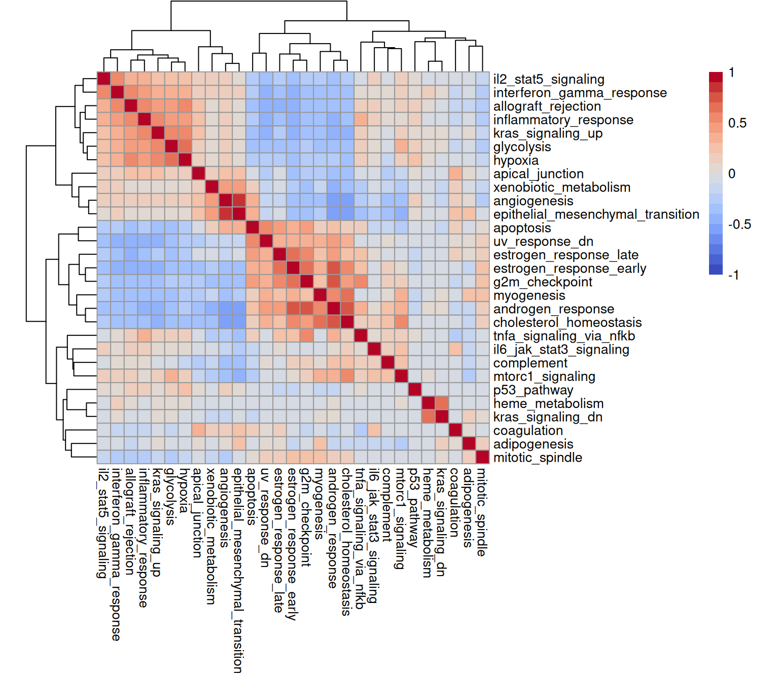
Highly correlated sets will exhibit similar spatial patterns. Let’s visualize some examples; here, hypoxia and myogenesis are spatially exclusive (they are negatively correlated and occupy separated ‘blocks’ in the correlation matrix displayed above), while apoptosis is ubiquitous (detected in >90% of cells).
Code
spe$in_tissue <- 1
lapply(c("hypoxia", "apoptosis", "myogenesis"), \(.) {
    q <- quantile(x <- spe[[.]], c(0.01, 0.99))
    x <- (x-q[1])/diff(q) # 01-quantile scaling
    x[x < 0] <- 0; x[x > 1] <- 1; spe[[.]] <- x
    # TODO: fix, cuz 'ggspaviz' is messing sth up...
    xy <- spatialCoordsNames(spe)
    xy <- match(xy, names(colData(spe)), nomatch=0)
    if (any(xy != 0)) colData(spe) <- colData(spe)[-xy]
    plt <- plotCoords(spe, annotate=.)
    plt$layers[[1]]$aes_params$stroke <- 0
    plt$layers[[1]]$aes_params$size <- 0.2
    plt
}) |>
    wrap_plots(nrow=1, guides="collect") &
    scale_color_gradientn(
        "q-scaled\nAUCell",
        colors=hcl.colors(9, "Plasma")) &
    theme(
        legend.key.height=unit(1, "lines"),
        legend.key.width=unit(0.5, "lines"),
panel.background=element_rect(fill="black")) 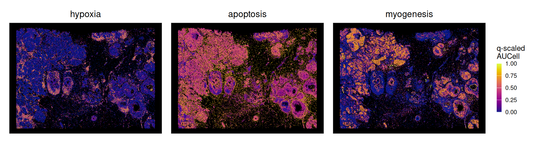
Lastly, we can aggregate signature scores by cell subpopulations. This can help us functionally characterize subpopulations that stem from, e.g., unsupervised approaches or in cases where the cells under study are poorly characterized.
Code
# aggregate AUC values by cluster
mu <- aggregateAcrossCells(auc, ids=colLabels(spe), use.assay.type="AUC", statistics="mean")
# visualize as (set x cluster) heatmap
pheatmap(mat=assay(mu), scale="row", col=pals::coolwarm())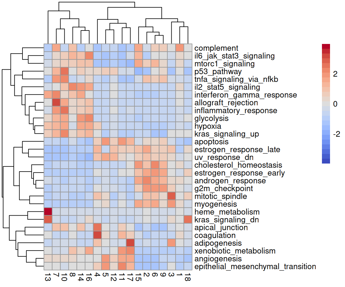
In a multi-sample setting - say, where sections across different stages of development, treatments, or health and disease - signatures may be compared between experimental conditions. Ideally, this’d be done at the subpopulation level, since compositional differences are deemed to drive differences (e.g., sections richer in CD8+ T cells are, by chance, more likely to score higher for cytotoxicity than sections where CD8+ T cells are absent, or similar).