7  Python interoperability

7.1 Introduction

Methods discussed in this book are usually available as either R or Python packages. Ideally, users should be able to leverage the full range of available tools for their analyses. Methods should be selected based on scientific merit (ideally demonstrated by neutral benchmarks), and independent of having been implemented in a given programming language (R or Python) or framework (e.g. Bioconductor or Seurat).

For single-cell and spatial omics data analysis, being able to leverage different ecosystems is especially powerful. On the one hand, Python offers superb infrastructure for image analysis and machine learning-based approaches. On the other hand, the R programming language has been historically dedicated to statistical computing; as a result, many modern R methods for spatial omics data build on a solid foundation of tools for spatial statistics and statistical modeling in general.

R’s application to statistical analysis of spatial data dates back decades, primarily in epidemiological and geospatial research. As a result, various tools for spatial analyses have been established. For example, sp provides a “coherent set of classes and methods for […] points, lines, polygons, and grids”; spatstat and, more recently, sf provide tools for spatial point pattern and vector data, respectively.

Different data structures, although standardized within a given framework, make switching between languages and tools somewhat cumbersome. In the realm of single-cell and spatial omics, all Bioconductor tools are built around SummarizedExperiment-derived classes, while Seurat (Hao et al. 2023), Giotto (Chen2023-Giotto-Suite?), and VoltRon each rely on their own object definitions. In Python, Scanpy (Wolf, Angerer, and Theis 2018) and Squidpy (Palla et al. 2022) use AnnData. Attempts to alleviate the problem are being made – e.g. zellkonverter, anndataR (Deconinck et al. 2025), and functions from Seurat allow for conversion between Python’s AnnData and R/Bioconductor’s SingleCellExperiment or SpatialExperiment.

On a higher level, tools that enable interoperability between programming languages have become available. For example, reticulate provides an R interface to Python, including support to translate between objects from both languages; basilisk facilitates Python environment management within the Bioconductor ecosystem, and can also be interfaced with reticulate; and Quarto can generate dynamic reports from code in different languages.

Quarto is the successor to R Markdown (by Posit, formerly known as RStudio). Similar to .Rmd files, .qmd files can include scientific content (e.g. cross-referencing, LaTeX-based equations), and can be published in multiple output formats (HTML, PDF, etc.). This book is built using Quarto.

In this chapter, we demonstrate examples showing how to set up Python environments and interact with anndata objects in R, using either a Conda environment or virtual environment, together with reticulate, basilisk, and/or zellkonverter.

7.2 Dependencies

library(SpatialExperiment)
library(VisiumIO)
library(OSTA.data)
library(jsonlite)
library(reticulate)
library(basilisk)
library(zellkonverter)

7.3 Conda environment and reticulate

In the first example, we set up a Conda environment and use reticulate to interact with Python anndata objects in R. This is the simplest option, and is the recommended starting point for most users. Note that we are using functions from the reticulate package in the code below.

To set up the Conda environment, we also need to specify which Python installation to use. In order to run this example programmatically to compile this book chapter, we install a new Python installation with Miniconda. However, if you are following this example on a laptop or another system, it is easier to specify an existing Python installation to use. This will help avoid cluttering your system with additional Python installations. This option is noted in the code comments below.

7.3.1 Install Miniconda

Note: skip this section if you are using an existing Python installation instead.

In order to build this book chapter programmatically, we install a new Python installation with Miniconda, which is a free, lightweight installation of Python, Conda, and a small number of packages, provided by Anaconda. Note that we also need to set some environment variables in R using Sys.setenv() to accept the terms of service prompt programmatically, which can also be skipped if you are installing Miniconda interactively.

# set environment variables to accept terms of service
Sys.setenv(CONDA_PLUGINS_AUTO_ACCEPT_TOS = "yes")
Sys.setenv(CI = "true")

# install Miniconda (or update if already installed)
if (dir.exists(miniconda_path())) {
  miniconda_update()
} else {
  install_miniconda()
}

7.3.2 Set up Conda environment

Next, we create a Conda environment and install some key dependencies.

If you are using an existing Python installation on your system (instead of installing Miniconda), this can be specified with the argument conda = ... – i.e. specify the path to the conda binary from the existing Python installation to use.

# create conda environment
env <- "py-interop"
conda_create(env, packages = "python=3.11")  # include 'conda = ...' argument to 
                                             # use an existing Python installation
use_condaenv(env, required = TRUE)

# list conda environments
conda_list()$name

##  [1] "base"         "py-interop"   "r-reticulate"

The following dependencies are needed in some of the following chapters, and need to be installed from conda-forge. This can also be skipped if you are only running the examples in this chapter. We install these dependencies here so that we can re-use this Conda environment again in later chapters.

# install dependencies that need to be installed from conda-forge 
# instead of PyPI
conda_install(
  envname = env, 
  packages = c("libcxx", "llvm-openmp", "llvmlite", "numba"), 
  channel = "conda-forge"
)

The following dependencies are necessary for the examples in this chapter. These are installed from PyPI.

# install Python packages from PyPI
conda_install(
  envname = env, 
  packages = c("Dask==2024.12.1", "zarr==2.18.7", "squidpy==1.6.2"), 
  pip = TRUE
)

The following option sets Python code chunks to run via reticulate, allowing this chapter to be compiled programmatically.

# set to run {python} code chunks via reticulate
knitr::opts_chunk$set(python.reticulate = TRUE)

7.3.3 SingleCellExperiment

7.3.3.1 Calling Python

After configuring the Python environment, R commands can now be run using reticulate as follows. For more details on the syntax used, see the reticulate documentation.

Note that running code in this way comes with a small overhead of starting up a Python session in the background. But this is typically small compared to the runtime required to run computation-heavy methods, or when analyzing large-scale single-cell and spatial data (hundreds of thousands of cells or more).

anndata <- import("anndata")

example_h5ad <- system.file("extdata", "krumsiek11.h5ad", 
                            package = "zellkonverter")
(ad <- anndata$read_h5ad(example_h5ad))

##  AnnData object with n_obs × n_vars = 640 × 11
##      obs: 'cell_type'
##      uns: 'highlights', 'iroot'

7.3.3.2 Continuing in R

We can access any of the variables above in R. For basic outputs, this works out of the box:

unique(ad$obs$cell_type)

##  [1] progenitor Mo         Ery        Mk         Neu       
##  Levels: Ery Mk Mo Neu progenitor

reticulate also supports a few direct type conversions (e.g. dictionary \(\leftrightarrow\) named list). In the example demonstrated here, we use zellkonverter to convert from AnnData to SingleCellExperiment:

(sce <- AnnData2SCE(ad))

##  class: SingleCellExperiment 
##  dim: 11 640 
##  metadata(2): highlights iroot
##  assays(1): X
##  rownames(11): Gata2 Gata1 ... EgrNab Gfi1
##  rowData names(0):
##  colnames(640): 0 1 ... 158-3 159-3
##  colData names(1): cell_type
##  reducedDimNames(0):
##  mainExpName: NULL
##  altExpNames(0):

7.3.3.3 Back to Python

We can also do the reverse, i.e. go from R’s SingleCellExperiment to Python’s AnnData:

(ad <- SCE2AnnData(sce, X_name = "X"))

##  AnnData object with n_obs × n_vars = 640 × 11
##      obs: 'cell_type'
##      uns: 'X_name', 'highlights', 'iroot'

7.3.4 SpatialExperiment

Since the SpatialExperiment class extends SingleCellExperiment (see Chapter 3), conversion operations that we discussed above are also applicable to SpatialExperiment. However, to accomplish a full conversion from the AnnData object, we need to manually insert the spatial information using reticulate directly.

7.3.4.1 Starting with R

For this use case with SpatialExperiment, we will use the dataset from Janesick et al. (2023), which includes Visium measurements on human breast cancer tissue.

id <- "Visium_HumanBreast_Janesick"
pa <- OSTA.data_load(id)
dir.create(td <- tempfile())
unzip(pa, exdir = td)
obj <- TENxVisium(
  spacerangerOut = file.path(td, "outs"), 
  format = "h5", 
  images = "lowres")
(spe <- VisiumIO::import(obj))

We also need to parse the original scaling information (i.e. scale factor) for spots and images available in the standard Visium output. We will use this later during conversion.

scalefactors <- jsonlite::read_json(file.path(td, "outs/spatial/scalefactors_json.json"))

We again use the SCE2AnnData function from zellkonverter from the previous example, and convert the SingleCellExperiment-relevant components of the SpatialExperiment object to an AnnData object.

(ad <- SCE2AnnData(spe, X_name = "counts"))

##  AnnData object with n_obs × n_vars = 4992 × 18085
##      obs: 'in_tissue', 'array_row', 'array_col', 'sample_id'
##      var: 'ID', 'Symbol', 'Type'
##      uns: 'X_name', 'resources', 'spatialList'
##      obsm: 'spatial'

We can now populate the uns and obsm components of the AnnData object with spatial coordinates and images. We start with the coordinates.

coords <- spatialCoords(spe)
colnames(coords) <- c("x", "y")
obsm <- list(spatial = coords)

Now let’s create the uns component. The list of uns should be composed of as many samples as the images in the SpatialExperiment object. Also, each sample entry in the list should have two elements, one for the image and the other for the scaling information.

# get image metadata
imgdata <- imgData(spe)

# get image
img <- imgRaster(spe)
img <- apply(img, c(1, 2), \(x) col2rgb(x))
img <- aperm(img, perm = c(2, 3, 1))
img <- img / 255

# create uns
uns <- list(
  spatial = setNames(list(NULL), imgdata$sample_id)
)
uns[["spatial"]][[imgdata$sample_id]] <- 
  list(images = list(lowres = img), 
       scalefactors = scalefactors)

Now let’s insert the components to the AnnData object, and write back to an .h5ad file.

ad$obs$library_id <- imgdata$sample_id
ad$obsm <- obsm
ad$uns <- uns
ad$write_h5ad("spe.h5ad")

7.3.4.2 Calling Python

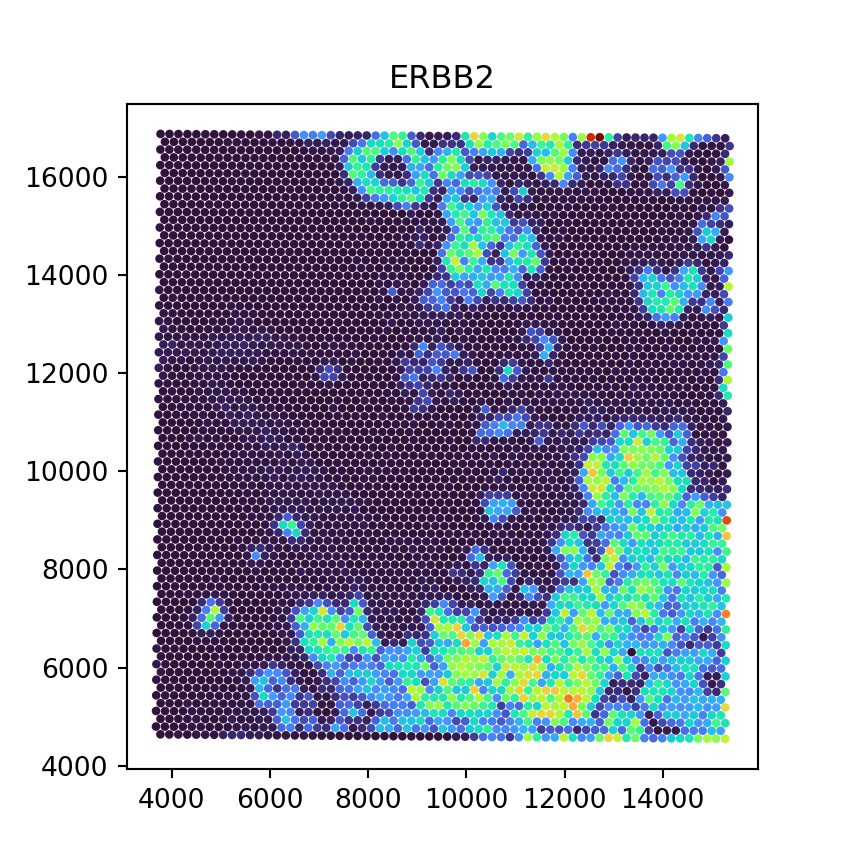
Now that we have converted the SpatialExperiment object to AnnData format, we can run Python code using the AnnData object. Here, for example, we visualize the Visium data using the squidpy module.

import squidpy as sq
import anndata as ad
import matplotlib.pyplot as plt

Read in spe.h5ad and visualize features or gene expression (e.g. ERBB2):

adata = ad.read_h5ad("spe.h5ad")
adata.var_names = adata.var['Symbol'].astype(str)
sq.pl.spatial_scatter(adata, 
                      color = ["ERBB2"], 
                      img_res_key = "lowres")
# plt.show() # needed to display plot if running code interactively

7.4 basilisk

Alternatively, we can use basilisk to install and manage Python environments. This is an alternative to setting up a Conda environment with an existing Python installation or a new installation of Miniconda, as demonstrated above. Using basilisk provides a self-contained environment, which helps avoid problems due to interactions with other environments on your system, and provides a higher level of reproducibility. This is also especially useful for package development by advanced users. However, setup may be more challenging in some cases.

7.4.1 Configuring Python

In this example, we use basilisk to create an environment containing a Python installation and all necessary dependencies for this chapter, and then use the resulting environment with reticulate, as above.

# set up environment using basilisk
env_basilisk <- BasiliskEnvironment(
  envname = "env-basilisk", 
  pkgname = "base", 
  packages = c("python=3.11", "Dask=2024.12.1"), 
  pip = c("zarr==2.18.7", "squidpy==1.6.2")
)

# use virtual environment
use_virtualenv(obtainEnvironmentPath(env_basilisk))

7.4.2 SingleCellExperiment

Now that we have set up the Python environment using basilisk, we can run R commands using reticulate in the same way as in the previous example. For example, using the same code as above:

anndata <- import("anndata")

example_h5ad <- system.file("extdata", "krumsiek11.h5ad", 
                            package = "zellkonverter")
(ad <- anndata$read_h5ad(example_h5ad))

To continue the example, please follow the code from the previous section above, starting from Section 7.3.3.

7.5 Appendix

Following are links to several key packages and tools relating to R-Python interoperability, which were mentioned in the sections above:

• anndataR (Deconinck et al. 2025): R package and community project to work with AnnData objects in R, including conversion to and from SingleCell/SpatialExperiment and Seurat objects

• zellkonverter (Zappia et al. 2020): R package to convert between AnnData and SingleCellExperiment objects, as well as reading from and writing to H5AD

• reticulate (Ushey, Allaire, and Tang 2017): R package and framework to call Python and run Python code in R, translate between R and Python objects, and manage virtual and Conda environments

• basilisk (Lun 2022): R package to install and manage Python environments in R packages and sessions

References

Deconinck, Louise, Luke Zappia, Robrecht Cannoodt, Martin Morgan, scverse core, Isaac Virshup, Chananchida Sang-Aram, et al. 2025. “anndataR Improves Interoperability Between r and Python in Single-Cell Transcriptomics.” bioRxiv. https://doi.org/10.1101/2025.08.18.669052.

Hao, Yuhan, Tim Stuart, Madeline H Kowalski, Saket Choudhary, Paul Hoffman, Austin Hartman, Avi Srivastava, et al. 2023. “Dictionary Learning for Integrative, Multimodal and Scalable Single-Cell Analysis.” Nature Biotechnology. https://doi.org/10.1038/s41587-023-01767-y.

Janesick, Amanda, Robert Shelansky, Andrew D. Gottscho, Florian Wagner, Stephen R. Williams, Morgane Rouault, Ghezal Beliakoff, et al. 2023. “High Resolution Mapping of the Tumor Microenvironment Using Integrated Single-Cell, Spatial and in Situ Analysis.” Nature Communications 14 (8353). https://doi.org/10.1038/s41467-023-43458-x.

Lun, Aaron. 2022. “Basilisk: A Bioconductor Package for Managing Python Environments.” Journal of Open Source Software 7. https://doi.org/10.21105/joss.04742.

Palla, Giovanni, Hannah Spitzer, Michal Klein, David Fischer, Anna Christina Schaar, Louis Benedikt Kuemmerle, Sergei Rybakov, et al. 2022. “Squidpy: A Scalable Framework for Spatial Omics Analysis.” Nature Methods 19: 171–78. https://doi.org/10.1038/s41592-021-01358-2.

Ushey, Kevin, Joseph J. Allaire, and Yuan Tang. 2017. “Reticulate: Interface to ’Python’.” R Package. https://doi.org/10.32614/CRAN.package.reticulate.

Wolf, F. Alexander, Philipp Angerer, and Fabian J. Theis. 2018. “SCANPY: Large-Scale Single-Cell Gene Expression Data Analysis.” Genome Biology 19 (15). https://doi.org/10.1186/s13059-017-1382-0.

Zappia, Luke, Aaron Lun, Jack Kamm, Robrecht Cannoodt, Gabriel Hoffman, and Marek Cmero. 2020. “anndataR Improves Interoperability Between r and Python in Single-Cell Transcriptomics.” R Package. https://doi.org/10.18129/B9.bioc.zellkonverter.