Code
library(BiocPkgTools)
foo <- tryCatch(
    biocExplore(),
error=\(e) NULL) # protect against unstable connectionThis chapter provides additional background about the Bioconductor ecosystem by exploring the space of packages that revolve around spatial and single cell omics data. We deliberately include the latter, since many tools developed for single cell data are either directly applicable to, or lay the foundation for tools developed for spatial data.
Here, we will rely on biocViews (Carey et al. 2025) that are provided in the DESCRIPTION of each package. These may be browsed online – in a non-programmatic manner – on the Bioconductor BiocViews website.
Note that the data reported herein may be inaccurate, since packages might provide inaccurate/incomplete biocViews. Especially the “Spatial” term relied upon here was added fairly recently and might be missing from older packages.
The BiocPkgTools package (Su et al. 2025) provides tools to access and explore Bioconductor package metadata in R, including their details (e.g., authors) and (monthly) download statistics.
biocExplore() provides an interactive way to explore the package space:
library(BiocPkgTools)
foo <- tryCatch(
biocExplore(),
error=\(e) NULL) # protect against unstable connectionbiocPkgList() retrieves the full Bioconductor software package listing (at the time of calling the function), including associated metadata. These include biocViews, which we can use to identify packages of interest:
# retrieve current package record
df <- biocPkgList()
# helper function to get indices of packages
# that contain 'biocViews' specified by 'x'
.f <- \(x, y=df) vapply(y$biocViews, \(.) all(x %in% .), logical(1))
# view "Spatial" packages
df$Package[.f("Spatial")]
## [1] "alabaster.sfe" "Banksy" "BatchSVG"
## [4] "Battlefield" "betaHMM" "BulkSignalR"
## [7] "CARDspa" "CatsCradle" "clustSIGNAL"
## [10] "concordexR" "CTSV" "cytoviewer"
## [13] "DenoIST" "DESpace" "escheR"
## [16] "FuseSOM" "GeomxTools" "ggsc"
## [19] "ggspavis" "HiCPotts" "HiSpaR"
## [22] "HistoImagePlot" "hoodscanR" "HuBMAPR"
## [25] "imcRtools" "jazzPanda" "knowYourCG"
## [28] "lisaClust" "miRspongeR" "mistyR"
## [31] "mitology" "MoleculeExperiment" "nnSVG"
## [34] "OSTA.data" "panoramic" "pengls"
## [37] "poem" "RankMap" "RegionalST"
## [40] "retrofit" "scatterHatch" "sccomp"
## [43] "scDesign3" "scFeatures" "scider"
## [46] "SEraster" "shinyDSP" "simpleSeg"
## [49] "smoothclust" "smoppix" "sosta"
## [52] "SpaceMarkers" "SpaceTrooper" "spacexr"
## [55] "SpaNorm" "spARI" "spaSim"
## [58] "SpatialArtifacts" "SpatialDecon" "SpatialExperiment"
## [61] "SpatialExperimentIO" "spatialFDA" "SpatialFeatureExperiment"
## [64] "spatialHeatmap" "SpatialOmicsOverlay" "spatialSimGP"
## [67] "SPIAT" "spicyR" "SpNeigh"
## [70] "spoon" "SpotClean" "SPOTlight"
## [73] "SpotSweeper" "standR" "Statial"
## [76] "stPipe" "SVP" "tidySpatialExperiment"
## [79] "tomoda" "tomoseqr" "tpSVG"
## [82] "VisiumIO" "visiumStitched" "Voyager"
## [85] "XeniumIO" "signifinder" "stJoincount"We can also browse for packages that also include more specific terms, for example:
# view "Spatial Clustering" packages
df$Package[.f(c("Spatial", "Clustering"))]
## [1] "Banksy" "clustSIGNAL" "concordexR" "FuseSOM"
## [5] "hoodscanR" "imcRtools" "poem" "smoothclust"
## [9] "spARI" "spatialHeatmap" "SPIAT" "stPipe"
## [13] "tomoda" "stJoincount"We will now have a look at the package ecosystem in a more quantitative manner. Specifically, we will investigate how the number of available packages evolves over time, and how long individual packages remain available (their “lifetime”). Lastly, we will quantify the number of times more specific subterms (co-)occur.
Let’s first summarize the number of packages available over time, focusing specifically on “SingleCell” and “Spatial” packages.
Note that we here rely on the first and last date at which a package was available through Bioconductor; some packages might have been deprecated at one point or another.
# dependencies
library(dplyr)
library(ggplot2)
# specify 'biocViews' of interest
names(ids) <- ids <- c("SingleCell", "Spatial")
now <- as.Date(format(Sys.Date(), "%Y-%m-%d"))
gg <- lapply(ids, \(id) {
    # get metadata & simplify naming
    nm <- df$Package[.f(id)]
    ys <- getPkgYearsInBioc(nm) |>
        mutate(first=first_version_release_date) |>
        mutate(last=last_version_release_date) |>
        mutate(last=case_when(is.na(last)~now, TRUE~last)) |>
        filter(!is.na(first))
    # complete months between first/last dates
    ys <- lapply(split(ys, ys$package), \(.) {
        data.frame(
            package=.$package,
            date=seq(.$first, .$last))
    }) |> do.call(what=rbind)
    # get cumulative number of packages available each month
    ys |> group_by(date) |> count()
}) |> bind_rows(.id="biocViews")ggplot(gg, aes(date, n, col=biocViews)) +
geom_line(linewidth=0.8) +
geom_smooth(data=filter(gg, n >= 5),
method="lm", se=FALSE, linewidth=1) +
scale_x_date(date_breaks = "1 year", date_labels = "%Y") +
labs(x=NULL, y="# packages") +
theme_bw() + theme(
aspect.ratio=1,
panel.grid.minor=element_blank(),
axis.text.x=element_text(angle=45, hjust=1))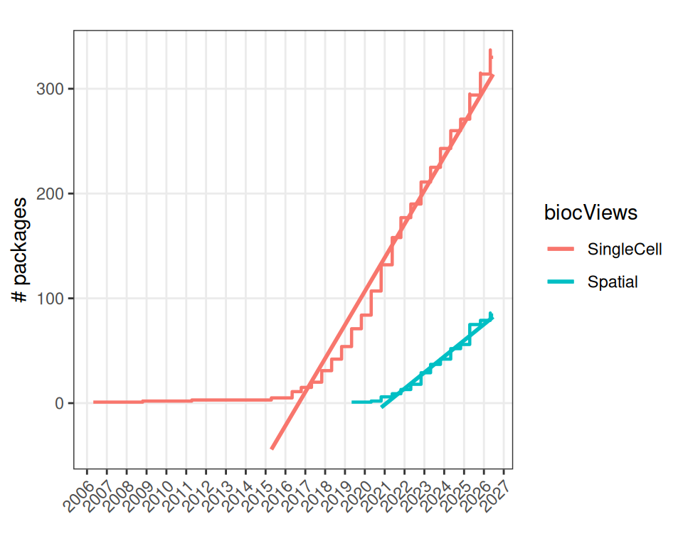
To get an idea of the project’s “growth” in this space, we can regress the number of packages against time using a linear model (LM). We here skip dates at which very few packages were available/being developed:
# fit linear model where x = 'date', y = # packages
# (starting at 'date' where at least 5 packages exist)
dy <- round(as.integer(diff(slice_min(group_by(.gg, biocViews), date)$date))/365, 2)
(bs <- .gg |>
    group_by(biocViews) |>
    group_split() |>
    # return coefficients = # packages
    # added each month (on average)
    sapply(\(.) coef(lm(n~date, .))[[2]]) |>
    setNames(sort(unique(gg$biocViews))))
## SingleCell Spatial
## 0.08785644 0.04196882The resulting coefficients tell us that about 1.05 single cell and 0.5 spatial packages are being added each year (on average), and there is a delay of about 5.54 years between them.
We can further inspect the “lifetime” of packages, i.e., how long they remain (installable) on Bioconductor:
A package will be deprecated if it fails to build and/or pass checks on the Bioconductor Build System (BBS), provided its maintainer is unresponsive and does not take action to fix the package before the next (six-monthly) release.
gg <- lapply(ids, \(id) {
    nm <- df$Package[.f(id)]
    ys <- BiocPkgTools:::getPkgYearsInBioc(nm)
}) |> bind_rows(.id="biocViews") |>
    mutate(years=approx_years_in) |>
    filter(!is.na(years))
mu <- gg |>
    group_by(biocViews) |>
    summarise_at("years", mean)
# print
cat("years in Bioconductor:\n")
summary(gg$approx_years_in)
# plot
ggplot(gg, aes(years, fill=biocViews)) +
    geom_histogram(alpha=1/3, binwidth=0.5) +
    geom_vline(
        linewidth=1, data=mu,
        aes(xintercept=years, col=biocViews)) +
    scale_x_continuous(breaks=seq(0, 100, 2)) +
    labs(x="lifetime (years)", y="# packages") +
    theme_bw() + theme(
        aspect.ratio=1,
        panel.grid.minor=element_blank(),
        axis.text.x=element_text(angle=45, hjust=1))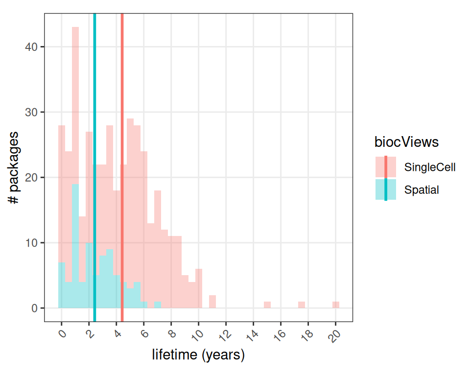
##  years in Bioconductor:
##     Min. 1st Qu.  Median    Mean 3rd Qu.    Max.
## 0.000 1.500 3.500 4.006 6.000 20.000Finally, let’s investigate more specific biocViews, e.g., the type of work tasks different packages cover. We will first count the number of packages that list specific terms that might be of interest in the context of single cell and spatial omics data analysis. Secondly, we will visualize their co-occurrence.
Note that packages can list an arbitrary number of terms so that packages can be counted in more than one category; e.g., “Visualization” appears in most.
i <- c("SingleCell", "Spatial")
j <- c(
    "BatchEffect", "Normalization", "QualityControl", "Visualization", # WorkflowStep
    "Clustering", "DimensionReduction", "FeatureExtraction", # StatisticalMethod
    "DifferentialExpression", "GeneSetEnrichment") # BiologicalQuestion
names(i) <- i; names(j) <- j
# count packages for each pair of terms
gg <- mapply(
    i=i, j=rep(j, each=2),
    SIMPLIFY=FALSE, \(i, j) {
        n <- sum(.f(c(i, j)))
        data.frame(i, j, n)
    }) |> do.call(what=rbind)
# order x-axis by total
xo <- gg |>
    group_by(j) |>
    summarise_at("n", sum) |>
    arrange(n) |>
    pull(j)
ggplot(gg, aes(j, n, fill=i)) +
    scale_x_discrete(limits=xo) +
    geom_col(position="dodge", alpha=2/3) +
    labs(x=NULL, y="# packages", fill="biocViews") +
    theme_bw() + theme(
        aspect.ratio=1,
        panel.grid.minor=element_blank(),
        axis.text.x=element_text(angle=45, hjust=1))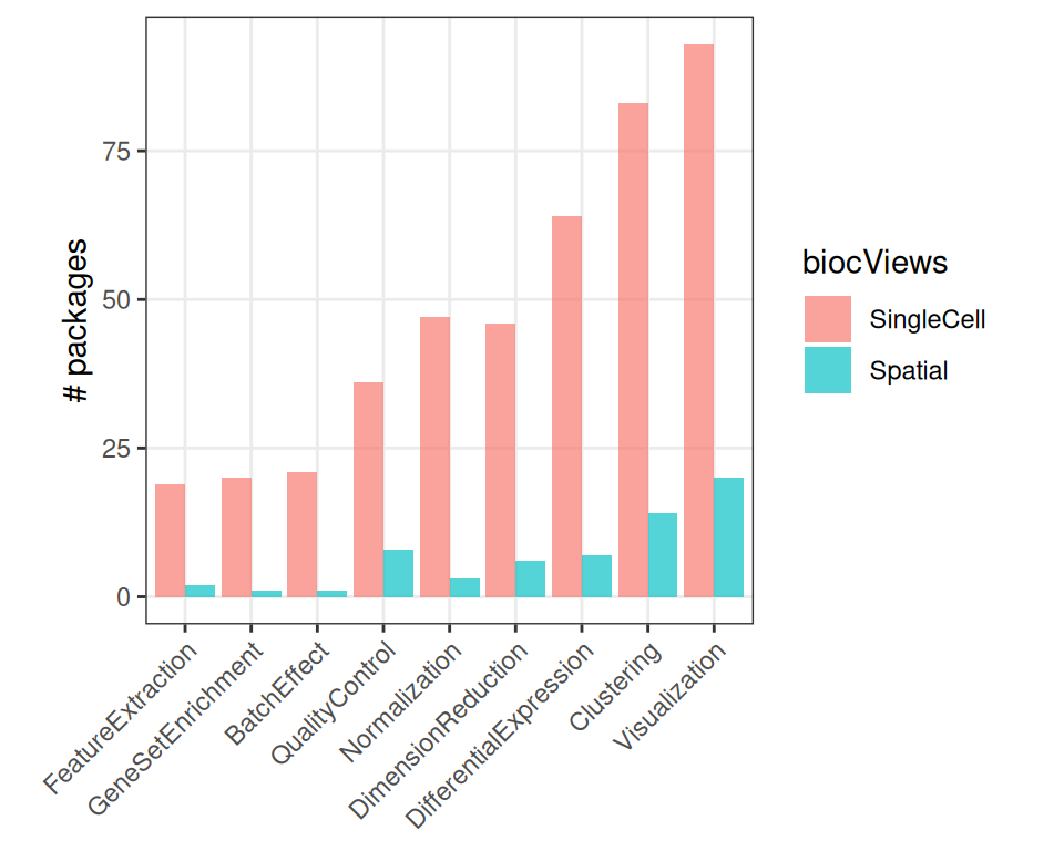
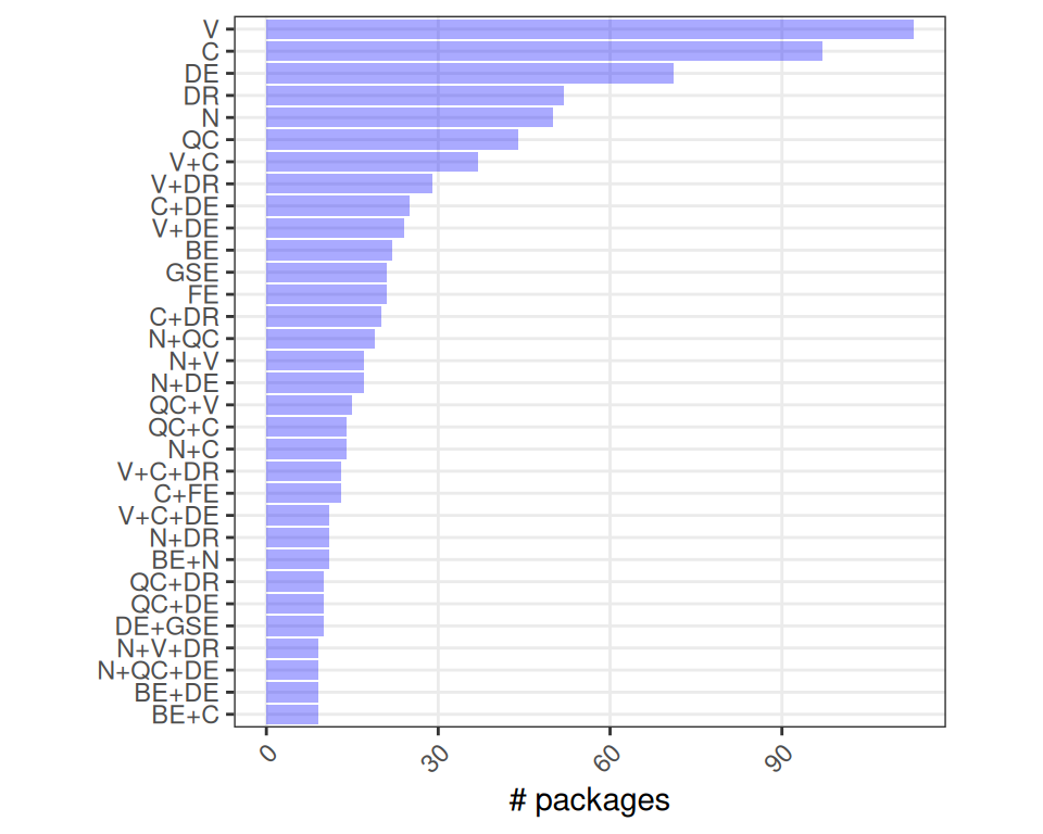
Because there are yet very few “Spatial” packages, we will pool “Spatial” and “SingleCell” tools when counting the number of times different terms appear together; i.e., biocViews contain “Spatial” OR “SingleCell”, together with “Clustering” AND “Visualization”, etc. (For concise labeling, we abbreviate biocViews to capital letters only; e.g., “BatchEffects” becomes “BE”.)
gg <- lapply(i, \(i) {
    lapply(seq_along(j), \(n) {
        js <- combn(j, n, simplify=FALSE)
        lapply(js, \(j) {
            n <- sum(.f(c(i, j)))
            j <- gsub("[a-z]", "", j)
            j <- paste(j, collapse="+")
            data.frame(i, j, n)
        }) |> do.call(what=rbind)
    }) |> do.call(what=rbind)
}) |> do.call(what=rbind) |>
    group_by(j) |>
    summarize_at("n", sum) |>
    slice_max(n, n=30)
yo <- gg$j[order(gg$n)]
ggplot(gg, aes(n, j)) +
    geom_col(alpha=1/3, fill="blue") +
    labs(y=NULL, x="# packages") +
    scale_y_discrete(limits=yo) +
    theme_bw() + theme(
        aspect.ratio=1,
        panel.grid.minor=element_blank(),
        axis.text.x=element_text(angle=45, hjust=1))