16 Workflow: Visium HD (segmented)

16.1 Preamble

16.1.1 Introduction

As of June 2025, Visium HD enables direct output of H&E-segmented cell-level data, in addition to the previous binned_outputs at 2, 8, and 16 µm, from SpaceRanger v4. This update simplifies the additional cell segmentation required when using bin2cell or StarDist. However, a comparative study of segmentation methods on Visium HD data has yet to be conducted.

The morphology-driven, nucleus-based segmentation produces polygons representing nuclei and cells across the entire tissue, as illustrated in the schematics provided by 10x Genomics.

16.1.2 Dependencies

Code

library(sf)
library(arrow)
library(dplyr)
library(tidyr)
library(scuttle)
library(SingleR)
library(Voyager)
library(ggplot2)
library(ggspavis)
library(VisiumIO)
library(OSTA.data)
library(patchwork)
library(SpotSweeper)
library(DropletUtils)
library(SpatialExperiment)
library(SpatialFeatureExperiment)
# set seed for random number generation
# in order to make results reproducible
set.seed(777)

Code

# utility for cropping by bounding box
.crop <- \(spe, box) {
    box <- as.list(box)
    xy <- spatialCoords(spe)
    spe[, 
        xy[,1] > box$xmin & xy[,1] < box$xmax &
        xy[,2] > box$ymin & xy[,2] < box$ymax ]
}

16.2 Setup

16.2.1 From SPE…

Analogous to other chapters, we start out by retrieving data files from the OSF repository using OSTA.data. Output files from SpaceRanger v4 are located under /segmented_outputs (see Chapter 5 for details on Visium HD output structure). We can read these cell-level data into R as a SpatialExperiment (Righelli et al. 2022) using VisiumIO’s TENxVisiumHD() function by specifying the segmented_outputs argument accordingly.

Code

# retrieve data from OSF repo
id <- "VisiumHD_HumanColon_Oliveira"
pa <- OSTA.data_load(id)
dir.create(td <- tempfile())
unzip(pa, exdir=td)

# read into 'SpatialExperiment'
seg <- file.path(td, "segmented_outputs")
spe <- TENxVisiumHD(
    format="h5", 
    images="lowres",
    segmented_outputs=seg) |>
    import()

# make gene symbols unique
gs <- rowData(spe)$Symbol
rownames(spe) <- make.unique(gs)

SpaceRanger also provides information on the mapping between binned outputs (2, 8, 16um) and segmented cells. These are provided in a separate .parquet file, which we can read using arrow’s read_parquet() function, and store as colData.

Code

# add bin-to-cell mapping information
map <- list.files(td, "mapping", full.names=TRUE)
head(map <- read_parquet(map))

##  # A tibble: 6 × 6
##    square_002um     square_008um    square_016um    cell_id         in_nucleus
##    <chr>            <chr>           <chr>           <chr>           <lgl>     
##  1 s_002um_00000_0… s_008um_00000_… s_016um_00000_… <NA>            FALSE     
##  2 s_002um_00000_0… s_008um_00000_… s_016um_00000_… <NA>            FALSE     
##  3 s_002um_00000_0… s_008um_00000_… s_016um_00000_… <NA>            FALSE     
##  4 s_002um_00000_0… s_008um_00000_… s_016um_00000_… cellid_0002449… FALSE     
##  5 s_002um_00000_0… s_008um_00000_… s_016um_00000_… cellid_0002449… FALSE     
##  6 s_002um_00000_0… s_008um_00000_… s_016um_00000_… cellid_0002449… FALSE     
##  # ℹ 1 more variable: in_cell <lgl>

Code

map_by_cell <- split(map, map$cell_id)
idx <- match(colnames(spe), names(map_by_cell))
spe$map <- map_by_cell[idx]
spe$in_tissue <- TRUE

Quick inspection shows us the percentage of 2um bins that were segmented, either as part of nuclei or whole cells:

Code

# percentage of segmented 2um bins
frac <- with(map, c(
    nuclear=mean(in_nucleus), 
    cellular=mean(in_cell)))
round(100*frac, digits=2)

##   nuclear cellular 
##     15.29    56.15

For runtime reasons, we will from the tissue to about half of its original width and height.

Code

xy <- spatialCoords(spe)
xs <- range(xy[, 1])
ys <- range(xy[, 2])
dx <- diff(xs)/4
dy <- diff(ys)/4
box <- list(
    xmin=xs[1]+dx, xmax=xs[2]-dx,
    ymin=ys[1]+dy, ymax=ys[2]-dy)
sub <- .crop(spe, box)

Code

# reverse y-coordinates of bounding box
.box <- box
.box$ymax <- -box$ymin
.box$ymin <- -box$ymax
aes <- list(col="red", fill=NA, linewidth=2)
plotCoords(
    spe[, sample(ncol(spe), 5e4)]) + 
    do.call(geom_rect, c(.box, aes)) +
plotCoords(
    sub[, sample(ncol(sub), 5e4)])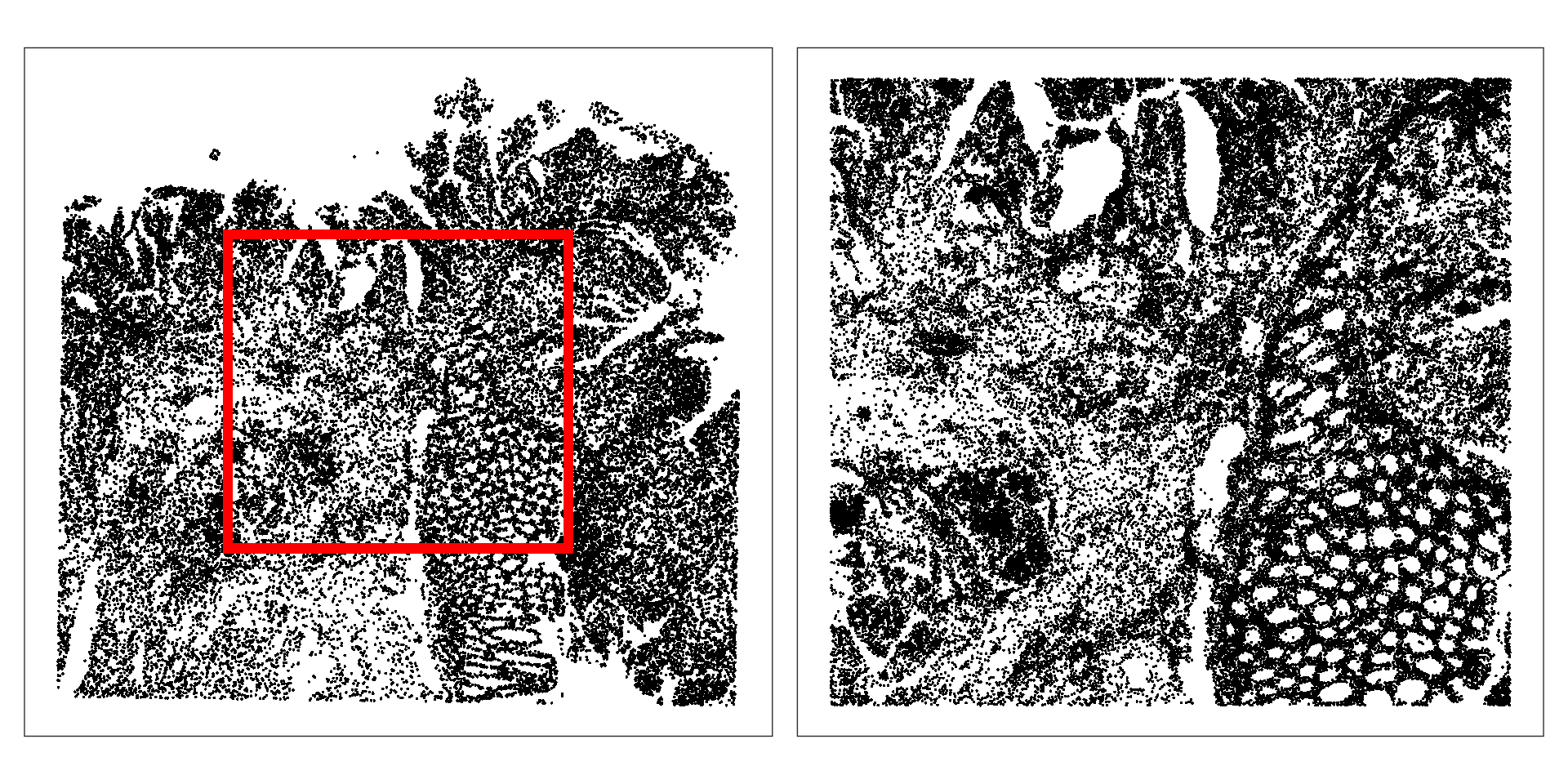

This retains about 28.55% of cells, and 63005 in total.

Code

round(100*ncol(sub)/ncol(spe), 2)

##  [1] 28.55

Code

ncol(spe <- sub)

##  [1] 63005

We also specify a much smaller region of interest (ROI) for visualization purposes.

Code

roi <- c(xmin=54e3, xmax=58e3, ymin=12e3, ymax=16e3)
spe$roi <- colnames(spe) %in% colnames(.crop(spe, roi))
plotCoords(spe, annotate="roi", point_size=0) + theme(legend.position="none")

16.2.2 …to SFE

Next, we will convert the above SPE into a SpatialFeatureExperiment (Moses et al. 2023) that allows us to also store cell segmentation masks as a colGeometry.

Code

ids <- gsub("cellid_(.*)-1", "\\1", colnames(spe))
spe$cell_id <- as.numeric(ids)

seg <- metadata(spe)$cellseg
idx <- match(spe$cell_id, seg$cell_id)
seg <- seg[idx, ]; rownames(seg) <- colnames(spe)

sfe <- toSpatialFeatureExperiment(spe)
colGeometries(sfe) <- list(cellseg=seg)

16.3 Exploratory

16.3.1 Cell masks

We can visualize such geometries using plot(st_geometry(x)) where x is the colGeometry of interest. As 63005 cells are a lot to visualize this way, we here crop() the data to filter for cells that fall within a small bounding box:

Code

# specify bounding box
box <- c(
    xmin=56e3, xmax=58e3,
    ymin=15e3, ymax=16e3)
# plot exemplary cell masks
geo <- colGeometry(crop(sfe, box))
plot(st_geometry(geo), col=rep(colors(), 2))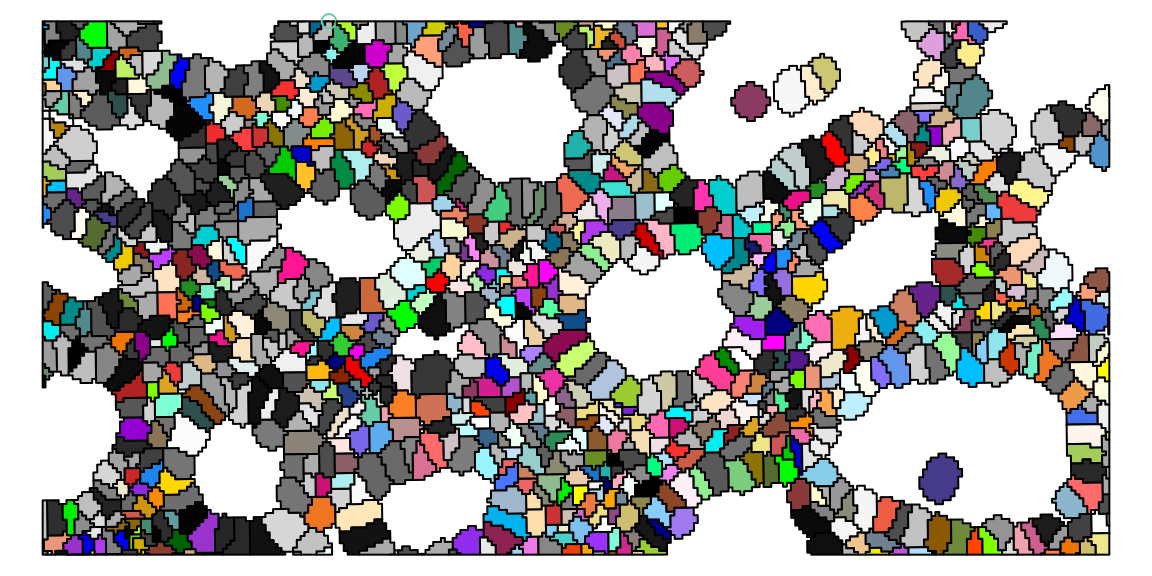

16.3.2 Bin mapping

We can estimate cell areas based on the number of 2um bins covered by each mask, e.g., 10 bins (2um\(^2\) each) would correspond to an area of 20um\(^2\). Based on this, we can also approximate the area of each cell’s nucleus using the in_nucleus flag provided in the bin-to-cell mapping information.

Code

# get cell areas = 2x number of 2um bins
sfe$um2 <- 2*sapply(sfe$map, nrow)
# get fraction of 2um bins that are nuclear
sfe$nuc <- sapply(sfe$map, \(.) mean(.$in_nucleus))
# get nucleus areas = cell area x nuclear fraction
sfe$nuc_um2 <- sfe$um2*sfe$nuc

We can also investigate the number of different cells that would be contained in 8um and 16um bins, respectively. Here, we can observe that 8/16um bins map to an average of about 2/4 cells, only 25% of bins map to more than 3/6 cells, and at most 9/20 cells are mapped to any bin.

Code

bin <- c("square_008um", "square_016um")
ncs <- lapply(bin, \(.) {
    idx <- split(seq(nrow(map)), map[[.]])
    sapply(idx, \(.) length(unique(map$cell_id[.])))
})
sapply(ncs, summary)

##              [,1]    [,2]
##  Min.    1.000000  1.0000
##  1st Qu. 1.000000  1.0000
##  Median  2.000000  4.0000
##  Mean    2.038471  3.9671
##  3rd Qu. 3.000000  6.0000
##  Max.    9.000000 20.0000

16.4 Quality control

16.4.1 Non-spatial

We can caluclate standard cell-level quality control metrics using scuttle’s addPerCellQCMetrics() function, specifying mitochondrial features as subsets of particular interest.

Code

sub <- list(mt=grep("^MT-", rownames(sfe)))
sfe <- addPerCellQCMetrics(sfe, subsets=sub)
sfe$log_sum <- log1p(sfe$sum)
head(colData(sfe)[c(
    "um2", "nuc_um2", "nuc",
    "sum", "subsets_mt_percent")])

##  DataFrame with 6 rows and 5 columns
##                           um2   nuc_um2       nuc       sum
##                     <numeric> <numeric> <numeric> <numeric>
##  cellid_000028786-1        26         8  0.307692       302
##  cellid_000028793-1        76        14  0.184211       290
##  cellid_000028794-1        38        14  0.368421       828
##  cellid_000028795-1        78        20  0.256410      1121
##  cellid_000028796-1        30        18  0.600000      1437
##  cellid_000028799-1        48        10  0.208333       488
##                     subsets_mt_percent
##                              <numeric>
##  cellid_000028786-1            2.31788
##  cellid_000028793-1            4.48276
##  cellid_000028794-1            3.86473
##  cellid_000028795-1            4.28189
##  cellid_000028796-1            7.23730
##  cellid_000028799-1            2.04918

Code

plotSpatialFeature(sfe[, sfe$roi], 
    colGeometryName="cellseg", 
    features="log_sum") +
    ggtitle("log-library size") +
plotSpatialFeature(sfe[, sfe$roi], 
    colGeometryName="cellseg", 
    features="subsets_mt_percent") +
    ggtitle("% mitochondrial") +
plot_layout(nrow=1) &
    theme(plot.title=element_text(hjust=0.5)) &
    scale_fill_gradientn(NULL, colors=pals::jet())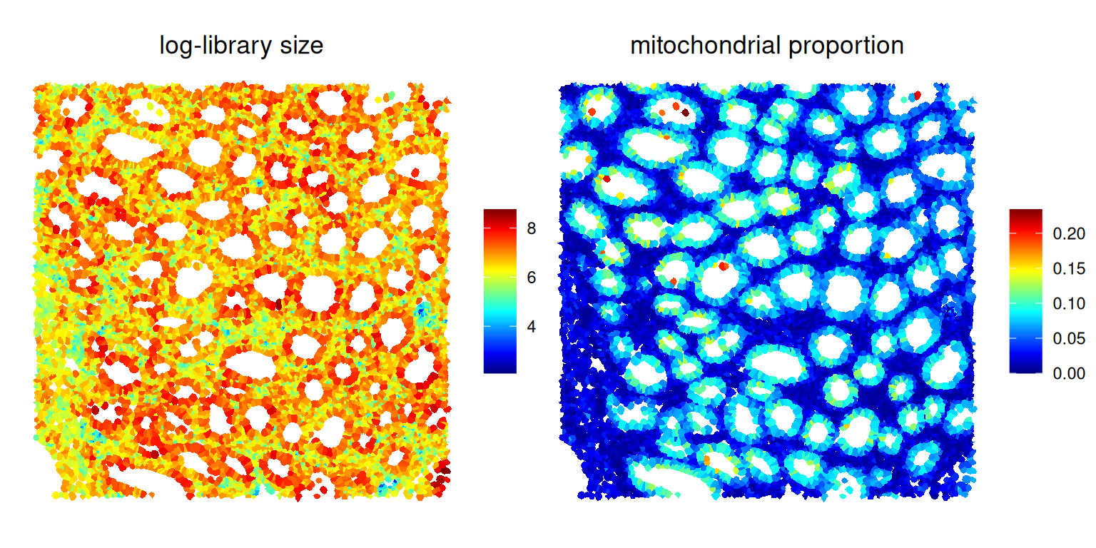

16.4.2 Spatially-aware

Spotsweeper (Totty, Hicks, and Guo 2025) determines outliers based on low log-library size, few uniquely detected features, or a high mitochondrial fraction compared to their surrounding neighborhood, which we recommend (see Chapter 10).

Code

# determine spatial outliers for different metrics
qc <- c("sum", "detected", "subsets_mt_percent")
for (. in qc) {
    sfe <- localOutliers(sfe, 
        workers=4, metric=., 
        log=TRUE, direction="lower")
}
# get cells x flags matrix
cd <- colData(sfe)
ol <- grep("outliers$", names(cd))
ol <- as.matrix(cd[ol])
# percentage of cells exluded for each 
round(100*colMeans(ol), 2)

##                 sum_outliers           detected_outliers 
##                         0.15                        0.17 
##  subsets_mt_percent_outliers 
##                         0.11

Code

# number of cells kept/removed overall
table(sfe$ex <- rowAnys(ol))

##  
##  FALSE  TRUE 
##  62805   200

We can visualize local outliers identified by SpotSweeper spatially. However, these are difficult to see, as only small cells were flagged.

Code

plotCoords(sfe[, order(sfe$ex)], 
    annotate="ex", point_size=0.2) +
    theme(legend.key.size=ggplot2::unit(0, "pt")) +
    scale_color_manual(values=c("grey90", "red")) +
    guides(col=guide_legend(override.aes=list(size=2)))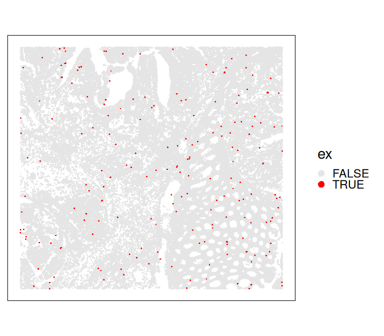

Code

# apply filtering
sfe <- sfe[, !sfe$ex]

16.5 Annotation

This Visium HD dataset provides matched scRNA-seq for the same tissue, which avoids tissue and batch effects that often complicate label transfer. colData slot Level1 contains broad, interpretable annotations that are well suited for label-transfer, deconvolution, and downstream interpretation. We will use these to map likely cell identities onto our Visium HD cells.

using deconvolution instead

We here use a single-cell label transfer approach to annotade cells. However, although each observation is intended to represent a single cell, there are still cases where this is not the case (e.g., as a result of partial volume effects at boundaries, segmentation errors, tightly packed regions, or local diffusion of transcripts.

Once could hence deconvolute cells instead (see Chapter 12), for example, using spacexr’s RCDT (Cable et al. 2022) in doublet mode to flag these cases and provide a principled estimate of the most likely composition. In practice, we expect most units to be classified as singlets, with a minority of doublets that warrant closer inspection or additional filtering.

Code

# retrieve single-cell reference from OSF repo
id <- "Chromium_HumanColon_Oliveira"
pa <- OSTA.data_load(id)
dir.create(td <- tempfile())
unzip(pa, exdir=td)

# read into 'SingleCellExperiment'
fs <- list.files(td, full.names=TRUE)
h5 <- grep("h5$", fs, value=TRUE)
sce <- read10xCounts(h5, col.names=TRUE)

# add cell metadata
csv <- grep("csv$", fs, value=TRUE)
cd <- read.csv(csv, row.names=1)
colData(sce)[names(cd)] <- cd[colnames(sce), ]

# use gene symbols as feature names
rownames(sce) <- make.unique(rowData(sce)$Symbol)

# exclude cells deemed to be of low-quality
sce <- sce[, sce$QCFilter == "Keep"]

# replace problematic characters
table(sce$Level1 <- gsub("\\s", "\\.", sce$Level1))

##  
##                B.cells           Endothelial            Fibroblast 
##                  33611                  7969                 28653 
##  Intestinal.Epithelial               Myeloid              Neuronal 
##                  22763                 25105                  4199 
##          Smooth.Muscle               T.cells                 Tumor 
##                  43308                 29272                 65626

For the purpose of this demo, we downsample to at most 1,000 cells per reference class. This preserves diversity within each class while keeping memory and runtime manageable.

Code

# (this is done only to keep runtime/memory low)
idx <- split(seq_len(ncol(sce)), sce$Level1)
idx <- lapply(idx, \(.) sample(., min(length(.), 1e3)))
ncol(.sce <- sce[, unlist(idx)])

##  [1] 9000

We next run BiocStyle::Biocpkg("SingleR") using Level1 (low-resolution) annotations and with argument aggr.ref=TRUE, such that reference profiles will be aggregated (per cluster) prior to annotation, and every cell will be assigned the label of the best-fitting pseudo-bulk scRNA-seq reference profile.

Code

# log-library size normalization
sfe <- logNormCounts(sfe)
.sce <- logNormCounts(.sce)
# perform label transfer at the Visium HD cell-level,
# using pseudo-bulk Chromium profiles as reference
res <- SingleR(test=sfe, ref=.sce, labels=.sce$Level1, aggr.ref=TRUE)
sfe$Level1 <- factor(res$pruned.labels)

Simplifying further, we can group cells into different compartments, namely, (malignant) tumor, immune, epithelial and stromal cells; we’ll see below that visualizing cells in this way nicely captures the general tissue structure.

Code

lab <- list(
    tum=c("Tumor"),
    epi=c("Intestinal.Epithelial"),
    imm=c("B.cells", "T.cells", "Myeloid"),
    str=c("Endothelial", "Fibroblast", "Smooth.Muscle"))
idx <- match(sfe$Level1, unlist(lab))
lab <- rep.int(names(lab), sapply(lab, length))
table(sfe$Level0 <- factor(lab[idx]))

##  
##    epi   imm   str   tum 
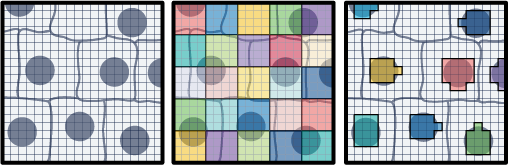
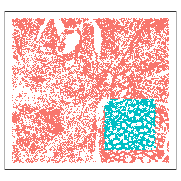
##   6915 11950 16120 27711

We can visualize low-resolution and compartment-level annotations over out ROI.

Code

pal_lv1 <- unname(pals::trubetskoy())
pal_lv0 <- c("gold", "turquoise", "deeppink", "navy")
plotSpatialFeature(sfe[, sfe$roi], 
    features="Level1", colGeometryName="cellseg") + 
    scale_fill_manual(values=pal_lv1) +
plotSpatialFeature(sfe[, sfe$roi], 
    features="Level0", colGeometryName="cellseg") + 
    scale_fill_manual(values=pal_lv0) +
plot_layout(nrow=1) &
    theme(legend.key.size=ggplot2::unit(.5, "lines"))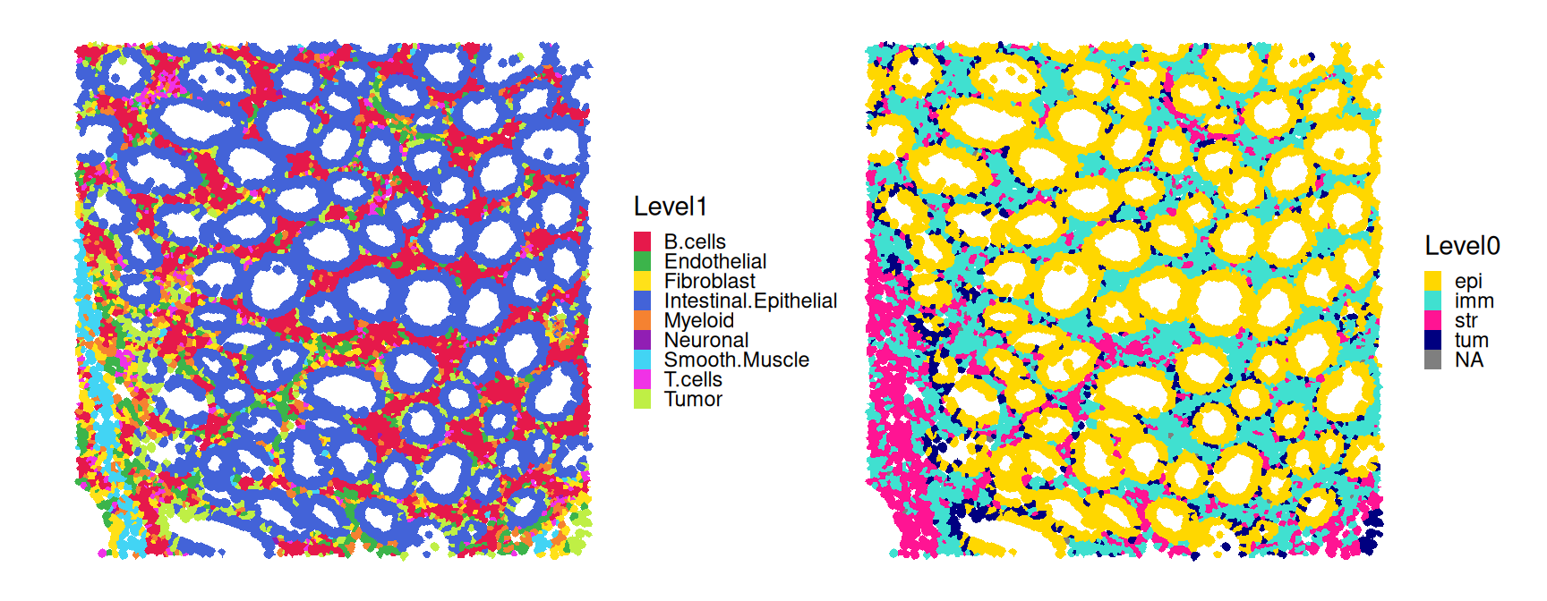

For whole-section visualization, we do not render segmentation boundaries but only cell centroids.

Code

plotCoords(sfe, 
    annotate="Level1", point_size=0.1) +
    scale_color_manual(values=pal_lv1) +
plotCoords(sfe, 
    annotate="Level0", point_size=0.1) +
    scale_color_manual(values=pal_lv0) +
plot_layout() &
    theme(legend.key.size=ggplot2::unit(0, "pt"))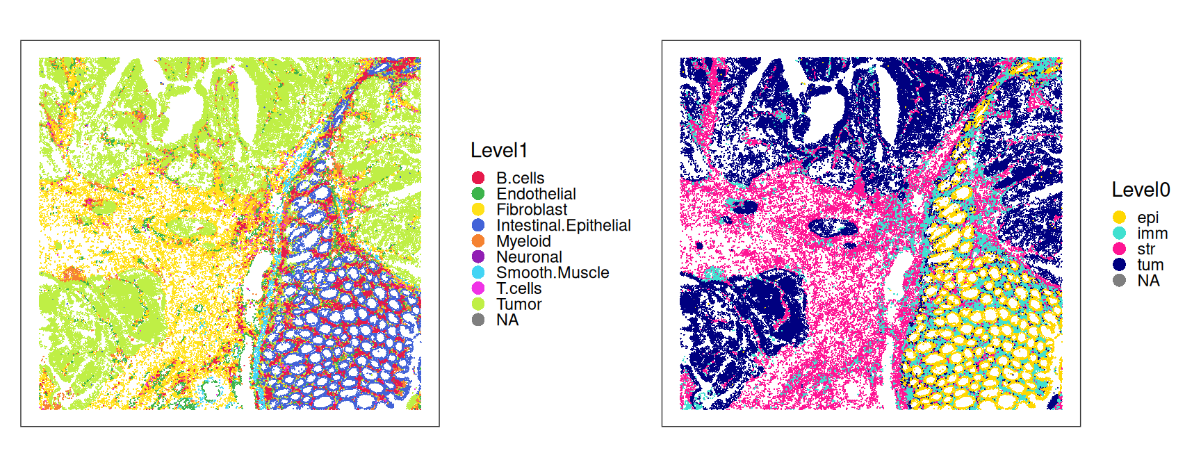

16.6 Downstream

Having annoted our cells, we can proceed with various downstream analyses. Compared to analysis at the bin-level, cell-level Visium HD data is similar to data from imaging-based platforms, but with full-transcriptome coverage. In princple, most analyses are thus transferable.

We refer readers to the chapters designed to specific analysis tasks, e.g., Chapter 29 on feature selection and testing, and Chapter 30 on feature-set scoring.

Instead, we quickly inspect how cell and nucleus areas differ across compartments and subpopulations. As expected, immune cells are smallest, tumor and structural cells (epithelial and stromal cells) tend to be larger.

Code

# wrangling
df <- data.frame(colData(sfe))
df <- filter(df, !is.na(Level0))
fd <- pivot_longer(df, ends_with("um2"))
fd$name <- factor(fd$name, labels=c("nuc.", "cell"))
ws <- c(nlevels(df$Level0), nlevels(df$Level1))
# plotting
ggplot(fd, aes(reorder(Level0, value), value, col=name)) +
ggplot(fd, aes(reorder(Level1, value), value, col=name)) + 
plot_layout(nrow=1, widths=ws, guides="collect") &
    geom_boxplot(key_glyph="point", outlier.size=0) &
    labs(col="area (um2)") & 
    theme_bw() & theme(
        axis.title=element_blank(),
        legend.key.size=ggplot2::unit(0, "pt"),
        axis.text.x=element_text(angle=45, hjust=1))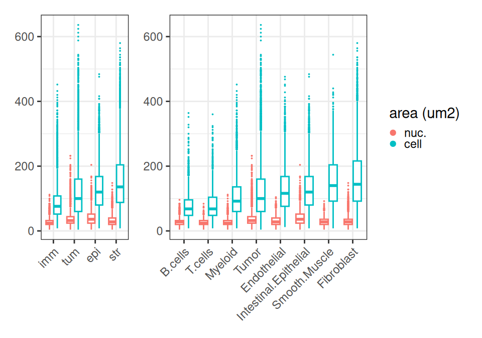

16.7 Appendix

This workflow is partly based on a workshop that has been taught at the European Bioconductor Conference 2025 (EuroBioC2025). Corresponding workshop material can be found here.

References

Cable, Dylan M, Evan Murray, Luli S Zou, Aleksandrina Goeva, Evan Z Macosko, Fei Chen, and Rafael A Irizarry. 2022. “Robust Decomposition of Cell Type Mixtures in Spatial Transcriptomics.” Nature Biotechnology 40 (4): 517–26. https://doi.org/10.1038/s41587-021-00830-w.

Moses, Lambda, Pétur Helgi Einarsson, Kayla Jackson, Laura Luebbert, A. Sina Booeshaghi, Sindri Antonsson, Nicolas Bray, Páll Melsted, and Lior Pachter. 2023. “Voyager: Exploratory Single-Cell Genomics Data Analysis with Geospatial Statistics.” bioRxiv. https://doi.org/10.1101/2023.07.20.549945.

Righelli, Dario, Lukas M Weber, Helena L Crowell, Brenda Pardo, Leonardo Collado-Torres, Shila Ghazanfar, Aaron T L Lun, Stephanie C Hicks, and Davide Risso. 2022. “SpatialExperiment: Infrastructure for Spatially-Resolved Transcriptomics Data in r Using Bioconductor.” Bioinformatics 38: 3128–31. https://doi.org/10.1093/bioinformatics/btac299.

Totty, Michael, Stephanie C. Hicks, and Boyi Guo. 2025. “SpotSweeper: Spatially Aware Quality Control for Spatial Transcriptomics.” Nature Methods 22: 1520–30. https://doi.org/10.1038/s41592-025-02713-3.