23 Spatially variable genes
23.1 Preamble
23.1.1 Introduction
Unsupervised clustering and label-transfer approaches yield (discrete, non-overlapping) grouping of cells by transcriptional – and presumably functional – similarity. Identifying differentially expressed genes (DEGs), i.e., genes that are up-/down-regulated in one or few subpopulation(s), helps characterize clusters (and, in an unsupervised setting, find biologically meaningful cluster labels).
By contrast, methods to identify spatially variable genes (SVGs) aim to find genes with spatially correlated patterns of expression. Feature selection in terms of SVGs can be used as a spatially-aware alternative to mean-variance relationship-based HVGs (c.f. Chapter 9), or to identify biologically informative genes as candidates for experimental follow-up.
Here, we demonstrate selected methods to identify SVGs de novo (using nnSVG), and based on pre-computed spatial clusters (using DESpace). We further compare these to DEGs as well as HVGs, and discuss the conceptual similarities and differences between genes identified through these different approaches.
23.1.2 Dependencies
23.2 Non-spatial
We can also use methods originally developed for bulk and single-cell transcriptomics, such as those for detecting highly variable genes (HVGs) and differentially expressed genes (DEGs), on spatial omics data. Note that HVGs are defined only based on molecular features (i.e., gene expression), and do not incorporate spatial information. In the context of single-cell and ST, differentially expressed (DE) may refer to differences between groups of samples, or to differences between clusters (e.g., cell types, or spatial domains); below, we consider changes across spatial structures.
23.2.1 Highly variable genes (HVGs)
For a comprehensive discussion on HVG selection, we refer readers to OSCA. Below, we take a standard approach for selecting HVGs. For more details and examples, see Chapter 9.
Code
# fit mean-variance relationship
dec <- modelGeneVar(spe)
23.2.2 Differentially expressed genes (DEGs)
For details on identifying DE genes between groups of cells from single-cell RNA-seq data, we refer readers to OSCA. Below, we show a potential approach, using marker detection methods on ST data, to identify DE genes between spatial clusters.
23.3 Spatially-aware
Here, we demonstrate brief examples of how to identify a set of top SVGs using (nnSVG (Weber et al. 2023) and DESpace (Cai, Robinson, and Tiberi 2024)). These methods are available through Bioconductor and can be easily integrated into Bioconductor-based workflows.
23.3.1 Spatially-variable genes (SVGs)
SVGs are usually identified integrating gene expression measurements with spatial coordinates, either with or without predefined spatial domains. SVGs approaches can be broadly categorized into three types: overall SVGs, spatial domain-specific SVGs, and cell type-specific SVGs (Yan, Hua, and Li 2024).
The detection of overall SVGs is sometimes used as a feature selection step for further downstream analyses such as spatially-aware clustering (see Chapter 22). Several methods have been proposed for detecting overall SVGs; below, we report some few notable examples:
- spatialDE (Svensson, Teichmann, and Stegle 2018) and nnSVG (Weber et al. 2023), which are based on a Gaussian process model;
- Moran’s I and Geary’s C, which ranks genes according to their observed spatial autocorrelation (see Chapter 25); and,
- SPARK (Sun, Zhu, and Zhou 2020; Zhu, Sun, and Zhou 2021), which uses a non-parametric test of the covariance matrices of the spatial expression data.
Spatial domain-specific SVGs target changes in gene expression between spatial domains, which are used to summarize the whole spatial information. Genes displaying expression changes across spatial clusters indicate SVGs. Spatial domains can be predefined based on morphology knowledge, or identified through spatially-aware clustering approaches such as BayesSpace (Zhao et al. 2021) and Banksy (Singhal et al. 2024). Methods that belong to this category include DESpace (Cai, Robinson, and Tiberi 2024) in R, and SpaGCN (Hu et al. 2021) in Python.
Cell type-specific SVG methods leverage external cell type annotations to identify SVGs within cell types. They analyze interaction effects between cell types and spatial coordinates (Yan, Hua, and Li 2024). Examplary methods in R include CTSV (J. Yu and Luo 2022), C-SIDE (implemented in spacexr; (Cable et al. 2022)), and spVC (S. Yu and Li 2024).
23.3.2 nnSVG
In this example, we use a small subset of the dataset for faster runtime. We select a subset of the data, by subsampling the set of spots and including stringent filtering for lowly expressed genes.
nnSVG using all spots for this dataset and default filtering parameters for an individual Visium sample from human brain tissue (available from spatialLIBD) takes around 45 minutes on a standard laptop.Code
# set random seed for number generation
# in order to make results reproducible
set.seed(123)
# sample 100 spots to decrease runtime in this demo
# (note: skip this step in full analysis)
n <- 100
sub <- spe[, sample(ncol(spe), 100)]
# filter lowly expressed genes using stringent
# criteria to decrease runtime in this demo
# (note: use default criteria in full analysis)
sub <- filter_genes(sub,     # filter for genes with...
    filter_genes_ncounts=10, # at least 10 counts in
    filter_genes_pcspots=3)  # at least 3% of spots
# re-normalize counts post-filtering
sub <- logNormCounts(sub)

# run nnSVG
set.seed(123)
sub <- nnSVG(sub)

# extract gene-level results
res_nnSVG <- rowData(sub)
# show results
head(res_nnSVG, 3)
## DataFrame with 3 rows and 17 columns
## gene_id gene_name feature_type sigma.sq
## <character> <character> <character> <numeric>
## ENSG00000162545 ENSG00000162545 CAMK2N1 Gene Expression 0.554287
## ENSG00000117632 ENSG00000117632 STMN1 Gene Expression 0.273690
## ENSG00000142937 ENSG00000142937 RPS8 Gene Expression 1.216073
## tau.sq phi loglik runtime mean
## <numeric> <numeric> <numeric> <numeric> <numeric>
## ENSG00000162545 6.26826e-01 5.62281 -141.482 0.009 1.95696
## ENSG00000117632 7.12078e-01 5.82105 -137.703 0.011 1.96579
## ENSG00000142937 3.66418e-05 43.88534 -150.198 0.024 1.70346
## var spcov prop_sv loglik_lm LR_stat rank
## <numeric> <numeric> <numeric> <numeric> <numeric> <numeric>
## ENSG00000162545 1.125278 0.380440 0.469292 -147.293 11.62212 30
## ENSG00000117632 0.994145 0.266129 0.277642 -141.098 6.78938 53
## ENSG00000142937 1.221055 0.647365 0.999970 -151.377 2.35774 80
## pval padj
## <numeric> <numeric>
## ENSG00000162545 0.00299425 0.0108791
## ENSG00000117632 0.03355091 0.0690009
## ENSG00000142937 0.30762644 0.4158654Code
# count significant SVGs (at 5% FDR significance level)
table(res_nnSVG$padj <= 0.05)
##
## FALSE TRUE
## 59 50Code
# identify the top-ranked SVGs
res_nnSVG$gene_name[res_nnSVG$rank == 1]
## [1] "MBP"Code
# store the top 7 SVGs
top_nnSVG <- res_nnSVG$gene_name[res_nnSVG$rank < 7.5]
23.3.3 DESpace
DESapce relies on pre-computed spatial domains to summarize the primary spatial structures of the data; see Chapter 22 on clustering.
Code
plotCoords(spe,
    annotate="BayesSpace") +
    theme(legend.key.size=unit(0, "lines")) +
    scale_color_manual(values=unname(pals::trubetskoy()))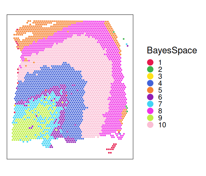
Code
##                          gene_id        LR   logCPM PValue FDR
##  ENSG00000123560 ENSG00000123560 18353.979 11.96618      0   0
##  ENSG00000197971 ENSG00000197971 28398.191 12.63393      0   0
##  ENSG00000150625 ENSG00000150625  4282.059 11.43082      0   0
##  ENSG00000163536 ENSG00000163536  2643.441 10.77555      0   0
##  ENSG00000269028 ENSG00000269028  5911.076 11.75599      0   0
##  ENSG00000143013 ENSG00000143013  2987.734 10.69452      0   0
Code
# count significant SVGs (at 5% FDR significance level)
table(res_DESpace$FDR <= 0.05)
##
## FALSE TRUE
## 2833 1258223.4 Downstream analyses
The set of top SVGs may be further investigated, e.g. by plotting the spatial expression of several top genes and via gene pathway analyses (i.e., comparing significant SVGs with known gene sets associated with specific biological functions).
23.4.1 Visualization
To visualize the expression levels of selected genes in spatial coordinates on the tissue slide, we can use plotting functions from the ggspavis package.
Code
# get top SVGs from each method
gs <- list(
    HVGs=top_HVGs,
    DEGs=top_DEGs,
    DESpace=top_DESpace)
# get gene symbols from ensembl identifiers
idx <- match(unlist(gs), rowData(spe)$gene_id)
.gs <- rowData(spe)$gene_name[idx]
# expression plots for each top gene
ps <- lapply(seq_along(.gs), \(.) {
    plotCoords(spe,
        point_size=0,
        annotate=.gs[.],
        assay_name="logcounts",
        feature_names="gene_name") +
        if (. %% 6 == 1) list(
            ylab(names(gs)[ceiling(./6)]),
            theme(axis.title.y=element_text()))
})
wrap_plots(ps, nrow=3) & theme(
    legend.key.width=unit(0.4, "lines"),
    legend.key.height=unit(0.8, "lines")) &
    scale_color_gradientn(colors = pals::parula())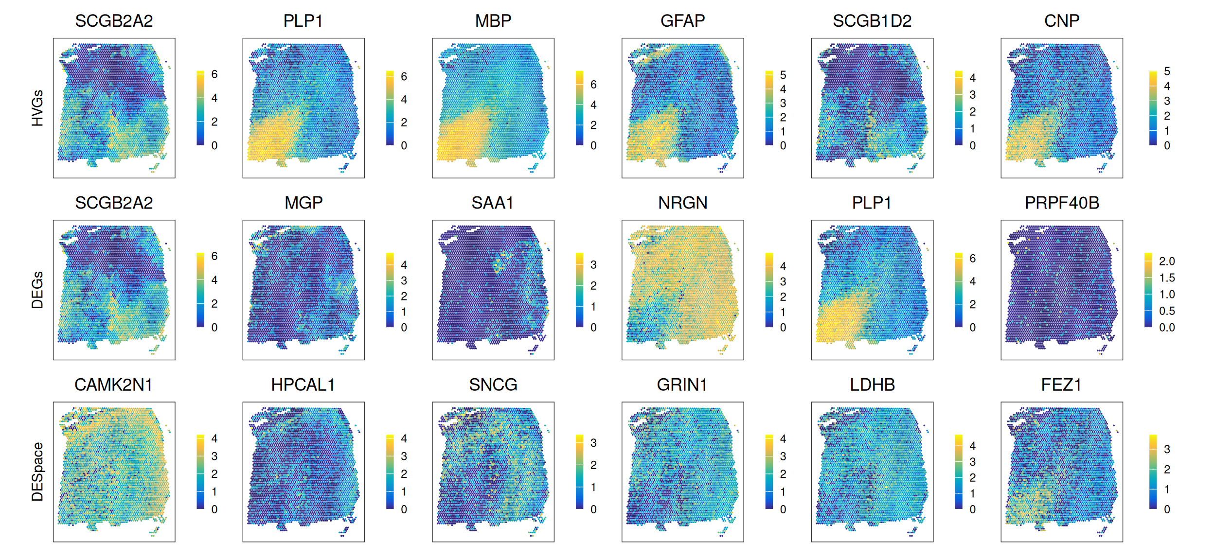
23.4.2 Comparison
We can compare the ranks of the genes detected by each method and compute pairwise correlations, highlighting two known cortical layer-associated SVGs: MOBP and SNAP25. While all four methods - HVGs, DEGs, SVGs identified through nnSVG and DESpace - yield similar gene ranks, each method captures distinct aspects of gene expression, with varying pairwise correlations between them.
Code
# subset data for the 113 genes nnSVG is based on
sub_gene <- rowData(sub)$gene_id
sub_DESpace <- res_DESpace[sub_gene, ]
sub_HVG <- as.data.frame(dec[sub_gene, ])

# aggregate DEGs for each spatial domain
subset_mgs <- lapply(mgs, \(x) x[sub_gene, 1:3] |> as.data.frame())
sub_DEG <- do.call(cbind, subset_mgs)
top_cols <- sub_DEG |> select(ends_with(".Top"))
sub_DEG$Top <- do.call(pmin, c(top_cols, na.rm = TRUE))

# compute ranks
sub_DESpace$rank <- rank(sub_DESpace$FDR, ties.method = "first")
sub_HVG$rank <- rank(-1 * sub_HVG$bio, ties.method = "first")
sub_DEG$rank <- rank(sub_DEG$Top, ties.method = "first")

# combine 'rank' column for each method
res_all <- list(
    nnSVG = as.data.frame(res_nnSVG),
    DESpace = sub_DESpace, HVGs = sub_HVG, DEGs = sub_DEG
)
rank_all <- do.call(cbind, lapply(res_all, `[[`, "rank"))
rank_all <- data.frame(gene_id = sub_gene, rank_all)
Code
# known SVGs for this data
known_genes <- c("MOBP", "SNAP25")
# method names
method_names <- c("nnSVG", "DESpace", "HVGs", "DEGs")
# convert data structure
rank_long <- rank_all |>
    left_join(data.frame(rowData(sub)[, c("gene_id", "gene_name")]), by = "gene_id") |>
    select(all_of(c("gene_name", method_names))) |>
    pivot_longer(cols = c(nnSVG, DESpace, HVGs, DEGs),
                 names_to = "method",
                 values_to = "rank")
# all pairwise comparisons
df_pairs <- t(combn(method_names, 2)) |> as.data.frame()
# function to plot each pairwise comparison
plot_pairwise_comparison <- function(m1, m2, df) {
  # filter the data for the two methods being compared
  df <- df |>
      filter(method %in% c(m1, m2)) |>
      pivot_wider(names_from = method, values_from = rank)
  # compute pearson correlation between methods
  cor_val <- cor(df[[m1]], df[[m2]], method = "spearman")
  # plot
  ggplot(df, aes(x = .data[[m1]], y = .data[[m2]])) +
      geom_point() +
      geom_text_repel(data = df %>% filter(gene_name %in% known_genes),
                      aes(label = gene_name), color = "red", size = 3.25,
                      nudge_x = 50, nudge_y = 10, box.padding = 0.5) +
      labs(x = paste(m1, "rank"), y = paste(m2, "rank"),
           title = paste(m2, "vs.", m1, ": Cor = ", round(cor_val, 2))) +
      #scale_color_manual(values = c("darkorange", "firebrick3", "deepskyblue2")) +
      theme_bw() + coord_fixed() +
      xlim(c(0, 120)) + ylim(c(0, 120))
}

# generate and display all pairwise comparison plots
plots <- lapply(seq_len(nrow(df_pairs)), \(i) {
    plot_pairwise_comparison(df_pairs[i, 2], df_pairs[i, 1],rank_long)
})

wrap_plots(plots, ncol = 3)
## Warning: Removed 1 row containing missing values or values outside the scale range
## (`geom_text_repel()`).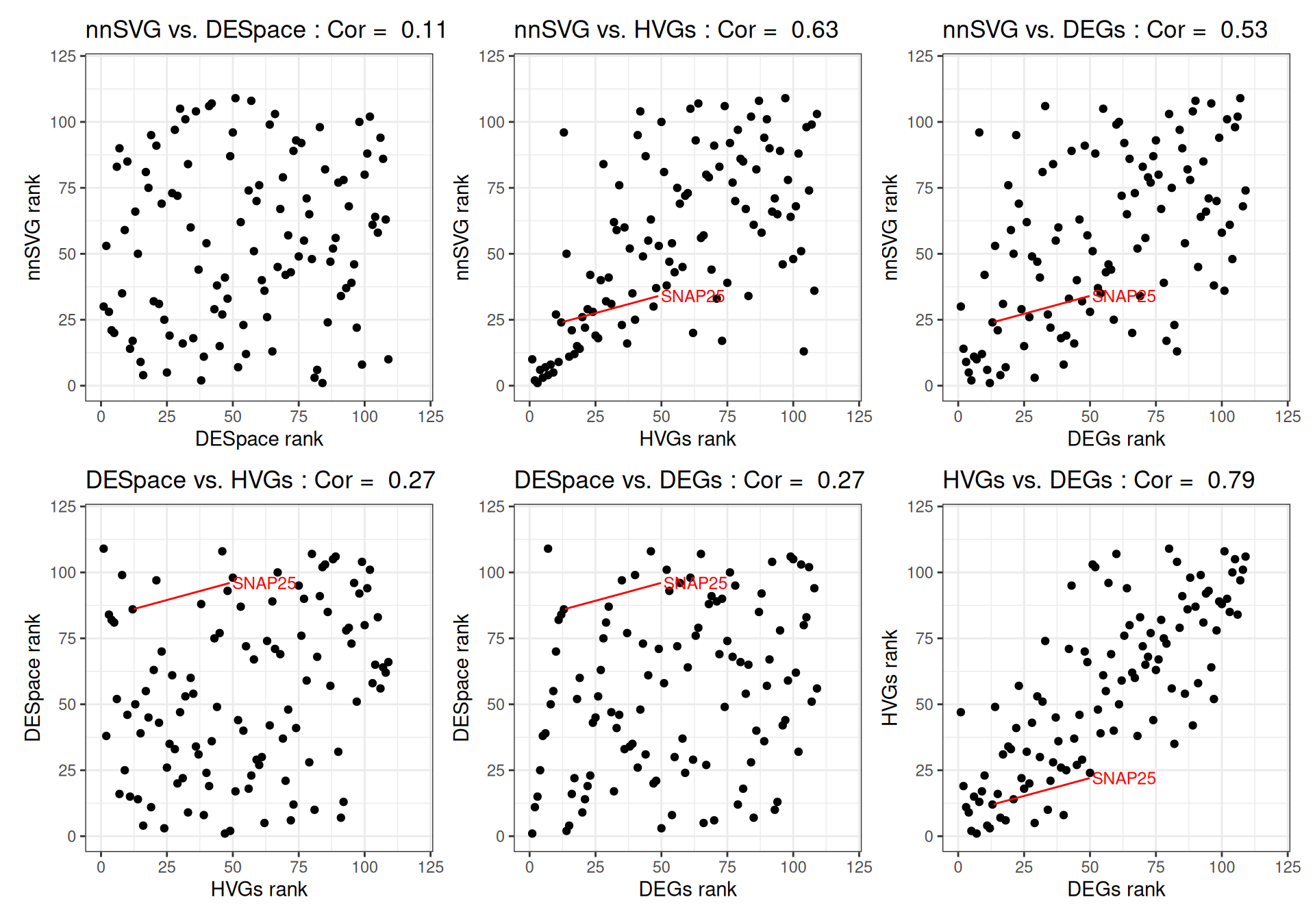
23.5 Appendix
Reviews
Benchmarks
- Li et al. (2023) compares 14 methods using 60 simulated datasets, generated using four different strategies, 12 experimental ST datasets, and 3 spatial ATAC-seq datasets.
- Chen, Kim, and Yang (2024) compares 8 methods based on 22 experimental datasets (8 technologies, 6 tissue types) and 9 datasets simulated using scDesign3 (Song et al. 2024).