library(SpatialExperiment)
spe <- readRDS("spe_hvgs.rds")
top_hvgs <- readRDS("top_hvgs.rds")9 Dimensionality reduction
9.1 Introduction
In this chapter, we apply dimensionality reduction methods to visualize the data and to generate inputs for further downstream analyses.
9.2 Load previously saved data
We start by loading the previously saved data object(s) (see Section 8.4).
9.3 Principal component analysis (PCA)
Apply principal component analysis (PCA) to the set of top highly variable genes (HVGs) to reduce the dimensionality of the dataset, and retain the top 50 principal components (PCs) for further downstream analyses.
This is done for two reasons: (i) to reduce noise due to random variation in expression of biologically uninteresting genes, which are assumed to have expression patterns that are independent of each other, and (ii) to improve computational efficiency during downstream analyses.
We use the computationally efficient implementation of PCA provided in the scater package (McCarthy et al. 2017). This implementation uses randomization, and therefore requires setting a random seed for reproducibility.
# compute PCA
set.seed(123)
spe <- runPCA(spe, subset_row = top_hvgs)

reducedDimNames(spe)
## [1] "PCA"dim(reducedDim(spe, "PCA"))## [1] 3524 509.4 Uniform Manifold Approximation and Projection (UMAP)
We also run UMAP on the set of top 50 PCs and retain the top 2 UMAP components, which will be used for visualization purposes.
# compute UMAP on top 50 PCs
set.seed(123)
spe <- runUMAP(spe, dimred = "PCA")

reducedDimNames(spe)
## [1] "PCA" "UMAP"dim(reducedDim(spe, "UMAP"))## [1] 3524 2# update column names for easier plotting
colnames(reducedDim(spe, "UMAP")) <- paste0("UMAP", 1:2)9.5 Save objects for later chapters
We also save the object(s) in .rds format for re-use within later chapters to speed up the build time of the book.
# save object(s)
saveRDS(spe, file = "spe_reduceddims.rds")
9.6 Visualizations
Generate plots using plotting functions from the ggspavis package. In the next chapter on clustering, we will add cluster labels to these reduced dimension plots.
# plot top 2 PCA dimensions
plotDimRed(spe, plot_type = "PCA")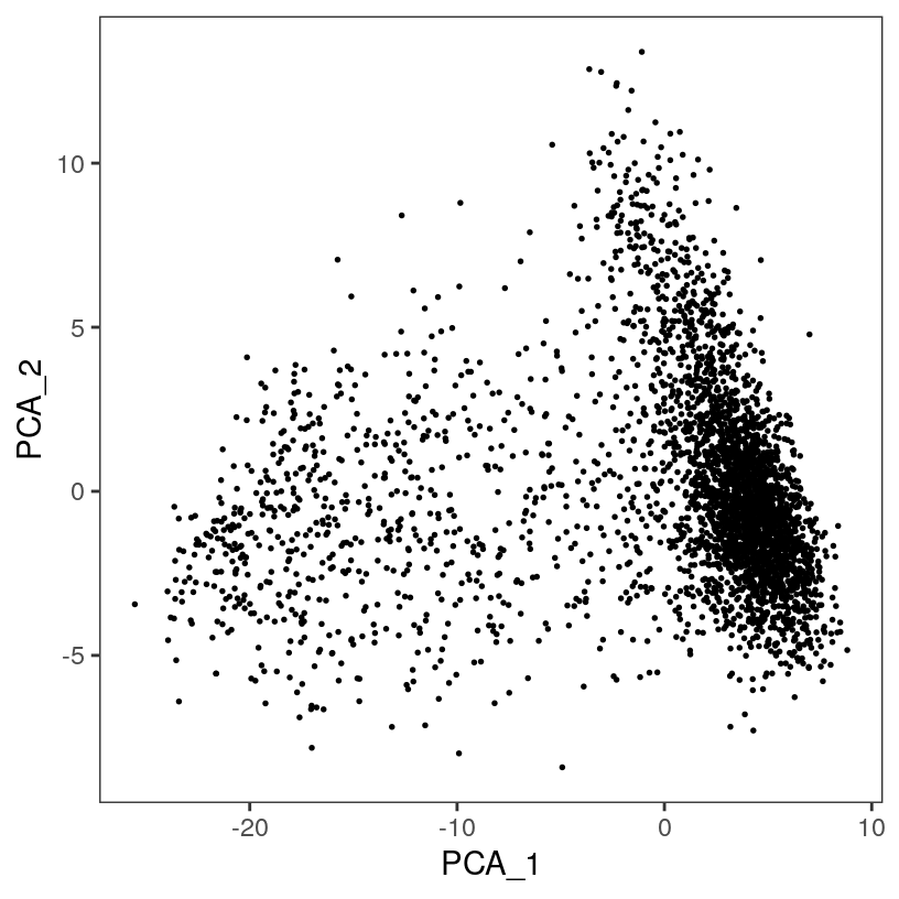
# plot top 2 UMAP dimensions
plotDimRed(spe, plot_type = "UMAP")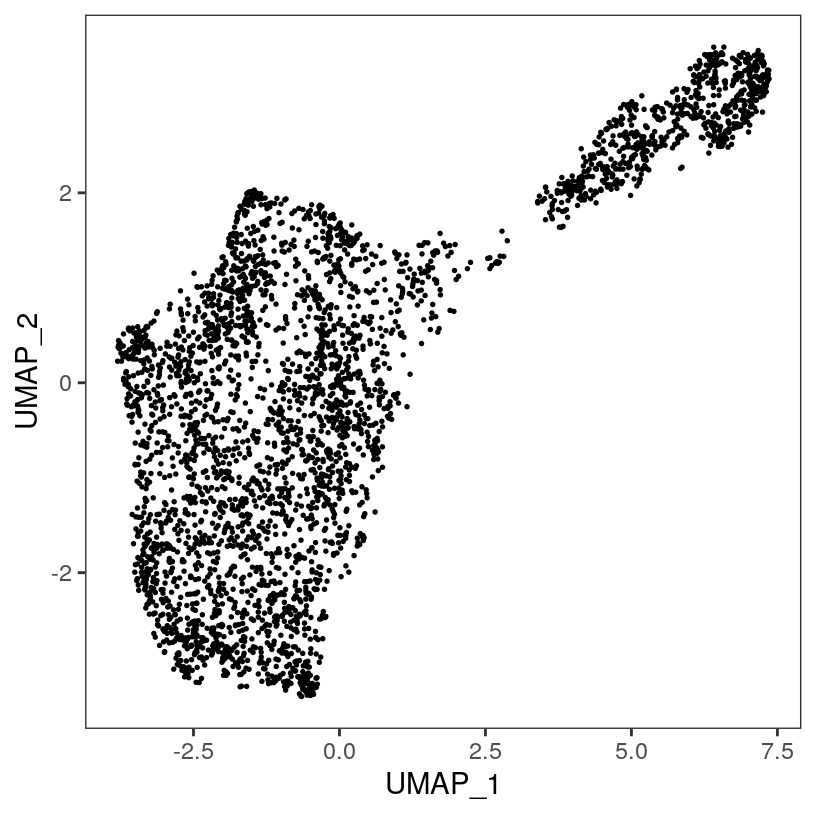
References
McCarthy, Davis J., Kieran R. Campbell, Aaron T. L. Lun, and Quin F. Wills. 2017. “Scater: Pre-Processing, Quality Control, Normalization and Visualization of Single-Cell RNA-seq Data in R.” Bioinformatics 33 (8): 1179–86. https://doi.org/10.1093/bioinformatics/btw777.