Best Practices for Spatial Transcriptomics Analysis with Bioconductor

4.1 Background

Here we apply normalization methods developed for scRNA-seq data, treating each spot as equivalent to one cell.

4.2 Previous steps

Code to run steps from the previous chapters to generate the SpatialExperiment object required for this chapter.

# LOAD DATA

library(SpatialExperiment)
library(STexampleData)
spe <- Visium_humanDLPFC()

# QUALITY CONTROL (QC)

library(scater)
# subset to keep only spots over tissue
spe <- spe[, colData(spe)$in_tissue == 1]
# identify mitochondrial genes
is_mito <- grepl("(^MT-)|(^mt-)", rowData(spe)$gene_name)
# calculate per-spot QC metrics
spe <- addPerCellQC(spe, subsets = list(mito = is_mito))
# select QC thresholds
qc_lib_size <- colData(spe)$sum < 600
qc_detected <- colData(spe)$detected < 400
qc_mito <- colData(spe)$subsets_mito_percent > 28
qc_cell_count <- colData(spe)$cell_count > 10
# combined set of discarded spots
discard <- qc_lib_size | qc_detected | qc_mito | qc_cell_count
colData(spe)$discard <- discard
# filter low-quality spots
spe <- spe[, !colData(spe)$discard]

4.3 Logcounts

Calculate log-transformed normalized counts (abbreviated as “logcounts”) using library size factors.

We apply the methods implemented in the scater (McCarthy et al. 2017) and scran (Lun, McCarthy, and Marioni 2016) packages, which were originally developed for scRNA-seq data, making the assumption here that these methods can be applied to SRT data by treating spots as equivalent to cells.

We use the library size factors methodology since this is the simplest approach, and can easily be applied to SRT data. Alternative approaches that are populare for scRNA-seq data, including normalization by deconvolution, are more difficulty to justify in the context of spot-based SRT data since (i) spots may contain multiple cells from more than one cell type, and (ii) datasets can contain multiple samples (e.g. multiple Visium slides, resulting in sample-specific clustering).

library(scran)

# calculate library size factors
spe <- computeLibraryFactors(spe)

summary(sizeFactors(spe))

   Min. 1st Qu.  Median    Mean 3rd Qu.    Max. 
 0.1321  0.6312  0.9000  1.0000  1.2849  3.7582

hist(sizeFactors(spe), breaks = 20)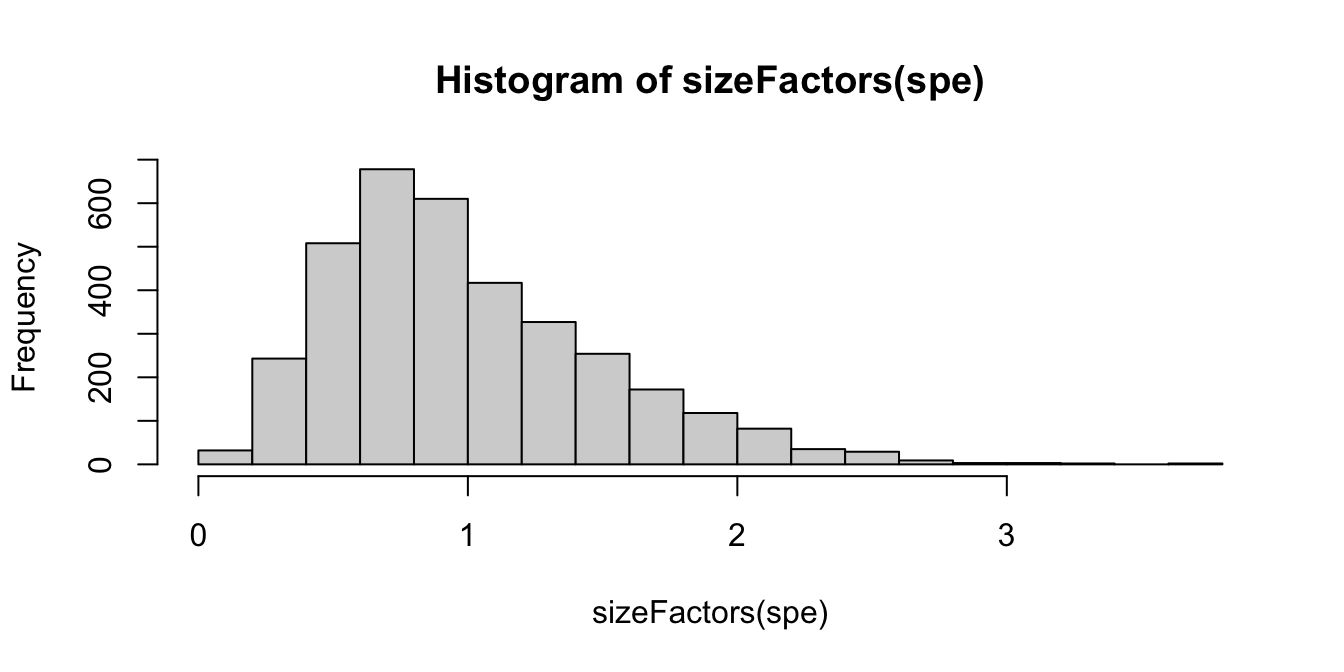

# calculate logcounts and store in object
spe <- logNormCounts(spe)

# check
assayNames(spe)

[1] "counts"    "logcounts"

dim(counts(spe))

[1] 33538  3524

dim(logcounts(spe))

[1] 33538  3524