6  Dimensionality reduction

6.1 Background

In this chapter, we apply dimensionality reduction methods to visualize the data and to generate inputs for further downstream analyses.

6.2 Previous steps

Code to run steps from the previous chapters to generate the SpatialExperiment object required for this chapter.

# LOAD DATA

library(SpatialExperiment)
library(STexampleData)
spe <- Visium_humanDLPFC()

# QUALITY CONTROL (QC)

library(scater)
# subset to keep only spots over tissue
spe <- spe[, colData(spe)$in_tissue == 1]
# identify mitochondrial genes
is_mito <- grepl("(^MT-)|(^mt-)", rowData(spe)$gene_name)
# calculate per-spot QC metrics
spe <- addPerCellQC(spe, subsets = list(mito = is_mito))
# select QC thresholds
qc_lib_size <- colData(spe)$sum < 600
qc_detected <- colData(spe)$detected < 400
qc_mito <- colData(spe)$subsets_mito_percent > 28
qc_cell_count <- colData(spe)$cell_count > 10
# combined set of discarded spots
discard <- qc_lib_size | qc_detected | qc_mito | qc_cell_count
colData(spe)$discard <- discard
# filter low-quality spots
spe <- spe[, !colData(spe)$discard]

# NORMALIZATION

library(scran)
# calculate logcounts using library size factors
spe <- logNormCounts(spe)

# FEATURE SELECTION

# remove mitochondrial genes
spe <- spe[!is_mito, ]
# fit mean-variance relationship
dec <- modelGeneVar(spe)
# select top HVGs
top_hvgs <- getTopHVGs(dec, prop = 0.1)

6.3 Principal component analysis (PCA)

Apply principal component analysis (PCA) to the set of top highly variable genes (HVGs) to reduce the dimensionality of the dataset, and retain the top 50 principal components (PCs) for further downstream analyses.

This is done for two reasons: (i) to reduce noise due to random variation in expression of biologically uninteresting genes, which are assumed to have expression patterns that are independent of each other, and (ii) to improve computational efficiency during downstream analyses.

We use the computationally efficient implementation of PCA provided in the scater package (McCarthy et al. 2017). This implementation uses randomization, and therefore requires setting a random seed for reproducibility.

# compute PCA
set.seed(123)
spe <- runPCA(spe, subset_row = top_hvgs)

reducedDimNames(spe)

[1] "PCA"

dim(reducedDim(spe, "PCA"))

[1] 3524   50

6.4 Uniform Manifold Approximation and Projection (UMAP)

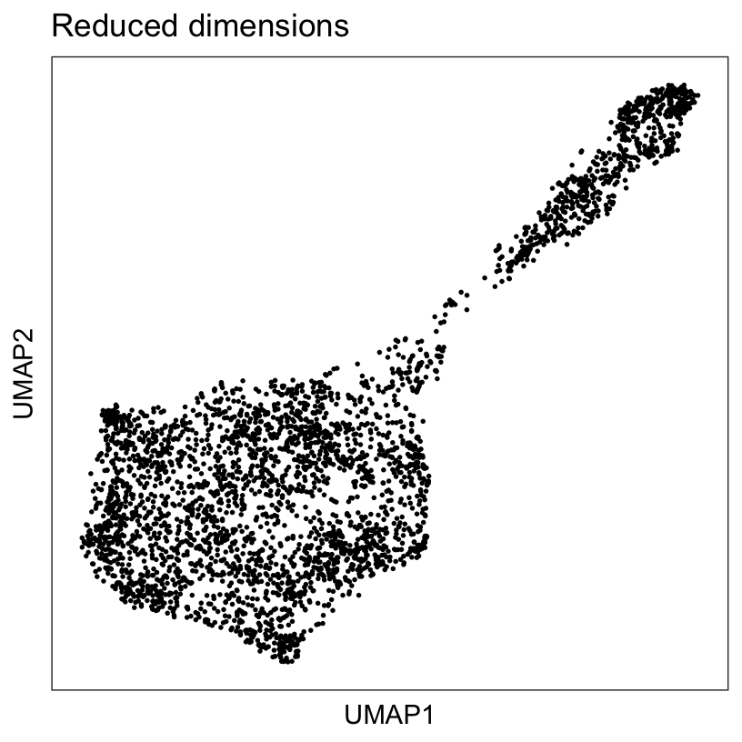
We also run UMAP (McInnes, Healy, and Melville 2018) on the set of top 50 PCs and retain the top 2 UMAP components, which will be used for visualization purposes.

# compute UMAP on top 50 PCs
set.seed(123)
spe <- runUMAP(spe, dimred = "PCA")

reducedDimNames(spe)

[1] "PCA"  "UMAP"

dim(reducedDim(spe, "UMAP"))

[1] 3524    2

# update column names for easier plotting
colnames(reducedDim(spe, "UMAP")) <- paste0("UMAP", 1:2)

6.5 Visualizations

Generate plots using plotting functions from the ggspavis package. In the next chapter on clustering, we will add cluster labels to these reduced dimension plots.

library(ggspavis)

# plot top 2 PCA dimensions
plotDimRed(spe, type = "PCA")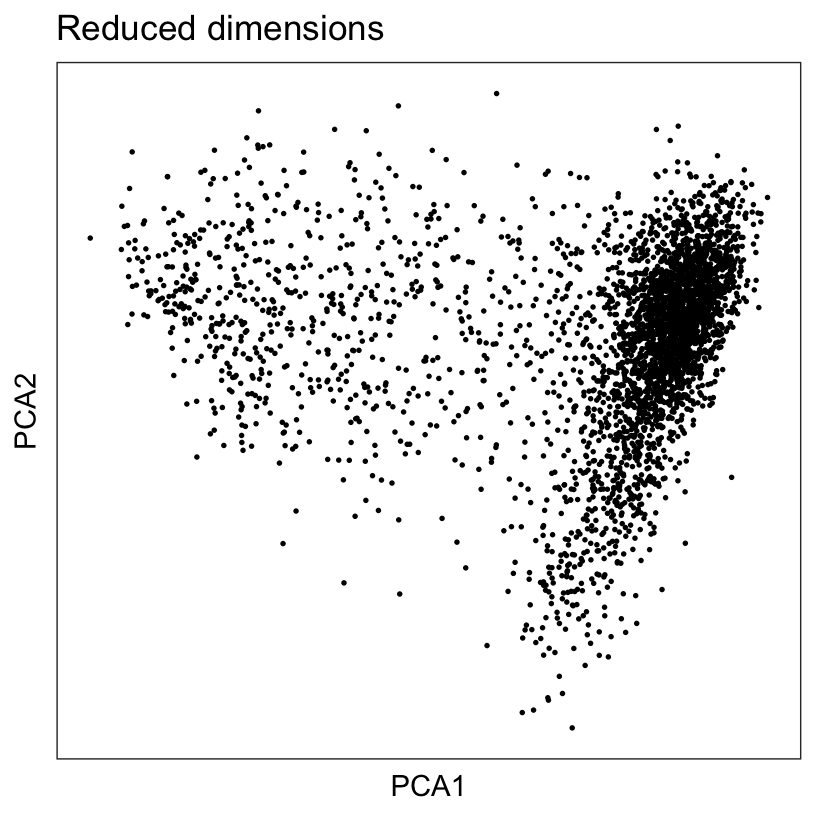

# plot top 2 UMAP dimensions
plotDimRed(spe, type = "UMAP")

McCarthy, Davis J, Kieran R Campbell, Aaron T L Lun, and Quin F Wills. 2017. “Scater: Pre-Processing, Quality Control, Normalization and Visualization of Single-Cell RNA-seq Data in R.” Bioinformatics 33 (8): 1179–86. https://doi.org/10.1093/bioinformatics/btw777.

McInnes, Leland, John Healy, and James Melville. 2018. “UMAP: Uniform Manifold Approximation and Projection for Dimension Reduction.” arXiv 1802.03426 (v2). https://arxiv.org/abs/1802.03426.