# LOAD DATA

library(SpatialExperiment)
library(STexampleData)
spe <- Visium_humanDLPFC()

# QUALITY CONTROL (QC)

library(scater)
# subset to keep only spots over tissue
spe <- spe[, colData(spe)$in_tissue == 1]
# identify mitochondrial genes
is_mito <- grepl("(^MT-)|(^mt-)", rowData(spe)$gene_name)
# calculate per-spot QC metrics
spe <- addPerCellQC(spe, subsets = list(mito = is_mito))
# select QC thresholds
qc_lib_size <- colData(spe)$sum < 600
qc_detected <- colData(spe)$detected < 400
qc_mito <- colData(spe)$subsets_mito_percent > 28
qc_cell_count <- colData(spe)$cell_count > 10
# combined set of discarded spots
discard <- qc_lib_size | qc_detected | qc_mito | qc_cell_count
colData(spe)$discard <- discard
# filter low-quality spots
spe <- spe[, !colData(spe)$discard]

# NORMALIZATION

library(scran)
# calculate logcounts using library size factors
spe <- logNormCounts(spe)

# FEATURE SELECTION

# remove mitochondrial genes
spe <- spe[!is_mito, ]
# fit mean-variance relationship
dec <- modelGeneVar(spe)
# select top HVGs
top_hvgs <- getTopHVGs(dec, prop = 0.1)

# DIMENSIONALITY REDUCTION

# compute PCA
set.seed(123)
spe <- runPCA(spe, subset_row = top_hvgs)
# compute UMAP on top 50 PCs
set.seed(123)
spe <- runUMAP(spe, dimred = "PCA")
# update column names
colnames(reducedDim(spe, "UMAP")) <- paste0("UMAP", 1:2)7 Clustering
7.1 Overview
Clustering is used in single-cell and spatial analysis to identify cell types.
Cell types and subtypes can be defined at various resolutions, depending on biological context. For the purposes of clustering, this means that the desired number of clusters also depends on biological context.
In the spatial context, we may be interested in e.g. (i) identifying cell types or subtypes that occur in biologically interesting spatial patterns, or (ii) identifying major cell types and performing subsequent analyses within these cell types.
7.2 Previous steps
Code to run steps from the previous chapters to generate the SpatialExperiment object required for this chapter.
7.3 Non-spatial clustering on HVGs
We can perform clustering by applying standard clustering methods developed for single-cell RNA sequencing data, using molecular features (gene expression). Here, we apply graph-based clustering using the Walktrap method implemented in scran (Lun et al. 2016), applied to the top 50 PCs calculated on the set of top HVGs.
In the context of spatial data, this means we assume that biologically informative spatial distribution patterns of cell types can be detected from the molecular features (gene expression).
# graph-based clustering
set.seed(123)
k <- 10
g <- buildSNNGraph(spe, k = k, use.dimred = "PCA")
g_walk <- igraph::cluster_walktrap(g)
clus <- g_walk$membership
table(clus)
clus
1 2 3 4 5 6 7
338 312 1146 978 274 116 360 # store cluster labels in column 'label' in colData
colLabels(spe) <- factor(clus)Visualize the clusters by plotting in (i) spatial (x-y) coordinates on the tissue slide, and (ii) reduced dimension space (PCA or UMAP). We use plotting functions from the ggspavis package.
For reference, we also display the ground truth (manually annotated) labels available for this dataset (in spatial coordinates).
From the visualizations, we can see that the clustering reproduces the known biological structure (cortical layers), although not perfectly. The clusters are also separated in UMAP space, but again not perfectly.
library(ggspavis)# plot clusters in spatial x-y coordinates
plotSpots(spe, annotate = "label",
palette = "libd_layer_colors")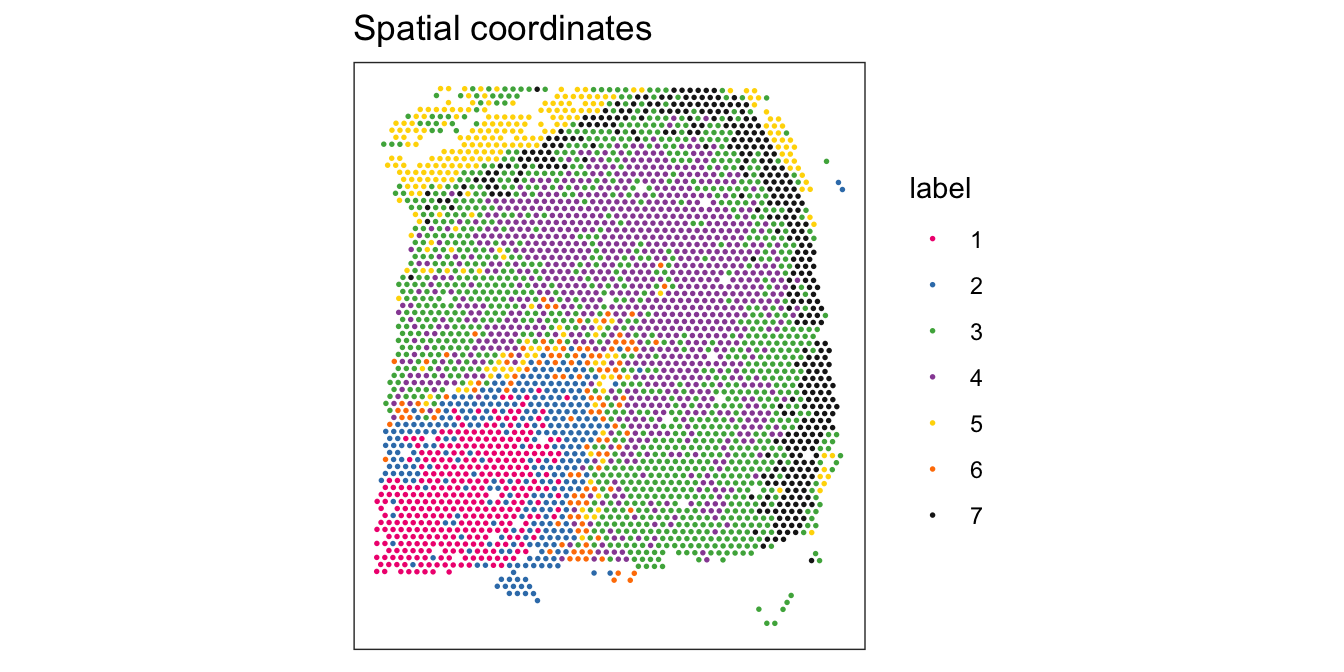
# plot ground truth labels in spatial coordinates
plotSpots(spe, annotate = "ground_truth",
          palette = "libd_layer_colors")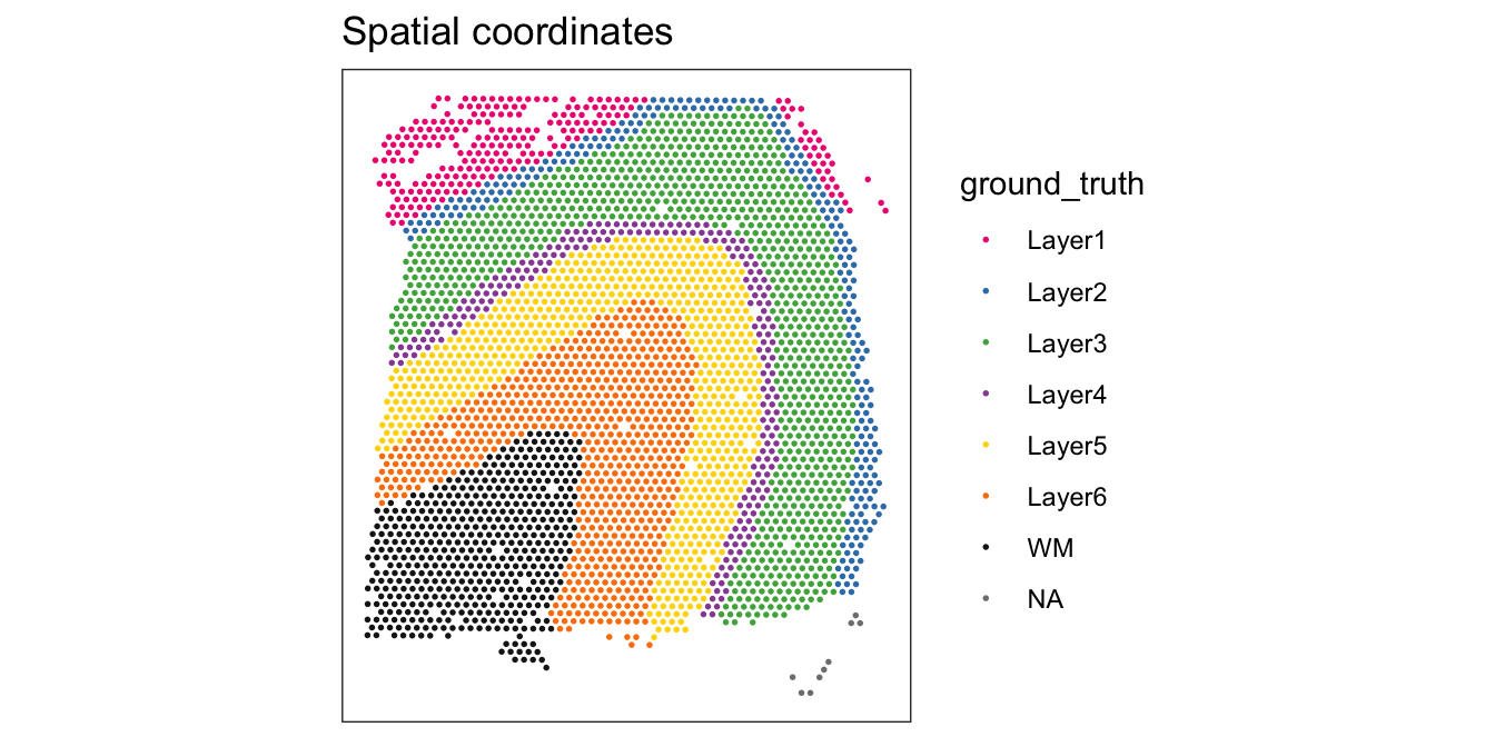
# plot clusters in PCA reduced dimensions
plotDimRed(spe, type = "PCA",
           annotate = "label", palette = "libd_layer_colors")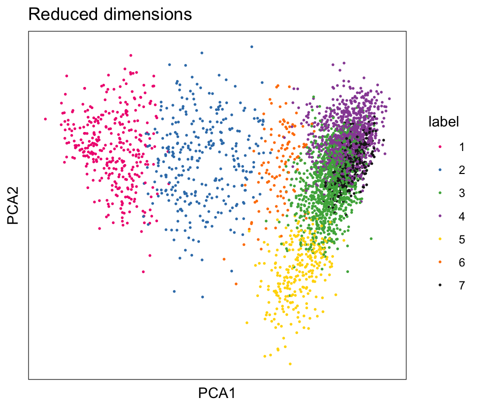
# plot clusters in UMAP reduced dimensions
plotDimRed(spe, type = "UMAP",
           annotate = "label", palette = "libd_layer_colors")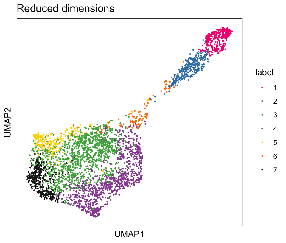
7.4 Spatially-aware clustering
In SRT data, we can also perform clustering that takes spatial information into account, for example to identify spatially compact or spatially connected clusters.
A simple strategy is to perform graph-based clustering on a set of features (columns) that includes both molecular features (gene expression) and spatial features (x-y coordinates). In this case, a crucial tuning parameter is the relative amount of scaling between the two data modalities – if the scaling is chosen poorly, either the molecular or spatial features will dominate the clustering. Depending on data availability, further modalities could also be included. In this section, we will include some examples on this clustering approach.
More sophisticated approaches for spatially-aware clustering include the following:
BayesSpace: available as an R package from Bioconductor and described by Zhao et al. (2021)
SpaGCN: available as a Python package from GitHub and described by Hu et al. (2021)
PRECAST: available as an R package from CRAN and described by Liu and Liao et al. (2023)