library(SpatialExperiment)
library(here)
spe <- readRDS(here("outputs/spe_qc.rds"))7 Normalization
7.1 Overview
Here we apply normalization methods developed for scRNA-seq data, treating each spot as equivalent to one cell.
7.2 Load data from previous steps
We start by loading the data object(s) saved after running the analysis steps from the previous chapters. Code to re-run the previous steps is shown in condensed form in Chapter 4.
7.3 Logcounts
Calculate log-transformed normalized counts (abbreviated as “logcounts”) using library size factors.
We apply the methods implemented in the scater (McCarthy et al. 2017) and scran (Lun, McCarthy, and Marioni 2016) packages, which were originally developed for scRNA-seq data, making the assumption here that these methods can be applied to SRT data by treating spots as equivalent to cells.
We use the library size factors methodology since this is the simplest approach, and can easily be applied to SRT data. Alternative approaches that are populare for scRNA-seq data, including normalization by deconvolution, are more difficulty to justify in the context of spot-based SRT data since (i) spots may contain multiple cells from more than one cell type, and (ii) datasets can contain multiple samples (e.g. multiple Visium slides, resulting in sample-specific clustering).
library(scran)

# calculate library size factors
spe <- computeLibraryFactors(spe)

summary(sizeFactors(spe))
Min. 1st Qu. Median Mean 3rd Qu. Max.
0.1321 0.6312 0.9000 1.0000 1.2849 3.7582 hist(sizeFactors(spe), breaks = 20)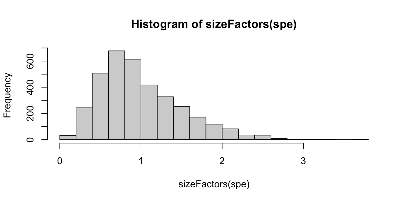
# calculate logcounts and store in object
spe <- logNormCounts(spe)

# check
assayNames(spe)
[1] "counts" "logcounts"dim(counts(spe))[1] 33538 3524dim(logcounts(spe))[1] 33538 3524